Cell embeddings and clusters across modalities

This tutorial embeds the same cells by their transcriptome and by their single-cell contact maps, clusters them, scores the clusters against published cell types (ARI / NMI) and lists marker features. It then embeds immunofluorescence (IF) signals that an imaging experiment measured at every DNA spot, and shows how the embeddings are stored so that the web browser can show them.

• Modules: uchrom.emb (embed_cells, normalize_counts, tfidf_lsi, cluster_cells, marker_features, scool_cell_features, aggregate_tracks; uchrom.emb.hic.schicluster_impute), chromdata.ChromData, uchrom_browser.data.

• Data: the scHiCAR mouse frontal cortex: RNA, ATAC and chromatin contacts measured in the same 5,313 nuclei, with 22 published cell types. Wei et al. 2026, Nat. Biotechnol., GEO GSE305439. The second dataset is the Takei et al. 2025 (Nature) cerebellum DNA seqFISH+ with 48 IF channels: replicate 1, 1,799 cells (Zenodo 7693825). Both are stores of the public U-Chrom atlas, read over HTTP: ds.atlas("schicar_mouse_cortex") (built by apps/atlas/recipes/build_schicar_mop.py, with embedded copies of the contact maps and of the RNA count matrix) and ds.atlas("takei2025_cerebellum") (built by apps/atlas/recipes/build_takei2025_cerebellum.py). They open backed: only the tables, contact maps and tracks the notebook uses are fetched, nothing has to be downloaded or built beforehand.

• Runtime: about 3 min on a laptop CPU with a good connection; about 2 min of it are reads over HTTP (the contact maps of section 6 and the IF tracks of section 8). We use 2,000 of the 5,313 scHiCAR cells, chosen at random, so that the contact-map step takes about a minute.

import time
import warnings
from pathlib import Path

import matplotlib.pyplot as plt
import numpy as np
import pandas as pd
import scipy.sparse as sp
from sklearn.decomposition import PCA
from sklearn.metrics import adjusted_rand_score, normalized_mutual_info_score
from sklearn.neighbors import NearestNeighbors

from chromdata import ChromData
import uchrom.datasets as ds
from uchrom import emb

plt.rcParams["figure.dpi"] = 90
warnings.filterwarnings("ignore", category=FutureWarning)
warnings.filterwarnings("ignore", message="IProgress not found")   # tqdm, imported by umap-learn

OUT = Path("_out"); OUT.mkdir(exist_ok=True)   # outputs: tutorials/_out/ (ignored by git)
T0 = time.time()

# small helpers used below: agreement scores and scatter plots
def agreement(labels, truth):
    return {"ARI": round(adjusted_rand_score(truth, labels), 3),
            "NMI": round(normalized_mutual_info_score(truth, labels), 3)}


def knn_purity(x, y, k=10):
    # fraction of each cell's k nearest neighbours (Euclidean) that share its label
    y = np.asarray(y)
    idx = NearestNeighbors(n_neighbors=k + 1).fit(x).kneighbors(x, return_distance=False)[:, 1:]
    return round(float((y[idx] == y[:, None]).mean()), 3)


def scatter(ax, xy, labels, title, palette=None, annotate=True, s=4):
    labels = pd.Series(labels).astype(str).to_numpy()
    cats = sorted(set(labels))
    palette = palette or dict(zip(cats, (plt.cm.tab20.colors + plt.cm.Dark2.colors) * 2))
    for c in cats:
        m = labels == c
        ax.scatter(xy[m, 0], xy[m, 1], s=s, lw=0, color=palette[c], label=c)
        if annotate:
            ax.text(*np.median(xy[m], axis=0), c, fontsize=6.5, ha="center", va="center", weight="bold")
    ax.set_title(title, fontsize=9)
    ax.set_xticks([]); ax.set_yticks([])

1. Load the scHiCAR store and pick the cells

The store holds no 3-D coordinates, so it has no spots. It holds one row per nucleus in cells, with the published cell_type, QC numbers, rna.<gene> counts and ATAC gene activity atac.<gene>. It also stores embeddings in cellm, and links to two files:

• a .scool file with one contact map per cell at 1 Mb;

• an .h5ad file with the full RNA count matrix.

A linked file normally stays outside the store (see the Linked modalities guide). An atlas store must stand alone on object storage, so it also carries embedded copies of its linked files (embedded/contacts/, embedded/anndata/). The link records stay in uns, and a reader uses the embedded copy when the file is not there: cd.linked_adata reads the AnnData, cd.load_linked_scool(key=..., cell=...) exports one cell’s map to a cooler file. This store also embeds the merged and per-cell-type pseudo-bulk maps (uns["linked_cool"]).

We keep 2,000 random cells and the published UMAP and cell types. We also keep atac_lsi, the ATAC embedding that the build recipe computed from 100 kb genome bins of all 5,313 cells. We use it for comparison, because the raw ATAC fragments (1.35 GB) are not needed here. Each cell type also gets a coarse class: excitatory neurons, inhibitory neurons or non-neuronal cells.

full = ds.atlas("schicar_mouse_cortex")       # backed, over HTTP: cells, cellm and uns are read at open
print(f"{full.n_cells:,} cells, {full.cells['cell_type'].nunique()} published cell types, "
      f"{sum(c.startswith('rna.') for c in full.cells.columns)} rna.* columns")
print("cellm:", list(full.cellm))
print("linked:", full.uns["linked_scool"]["per_cell"]["path"], "and", full.uns["linked_anndata"]["path"])
embedded = full.embedded_links()
print(f"embedded copies: {len(embedded['contacts'])} contact maps (per_cell, all_cells and one per cell type), "
      f"{len(embedded['anndata'])} AnnData")

N_CELLS = 2000
keep = np.sort(np.random.default_rng(0).choice(full.n_cells, N_CELLS, replace=False))

CLASS = {**dict.fromkeys(["L23IT.1", "L23IT.2", "L23IT.3", "L45IT", "L5IT", "L6IT", "L6CT", "L56NP", "PT", "CLA"],
                         "excitatory"),
         **dict.fromkeys(["Pvalb", "Sst", "Vip", "Lamp5", "D2MSN"], "inhibitory"),
         **dict.fromkeys(["Astro", "Oligo", "OPC", "MGL", "Endo", "Peri", "LMC"], "non-neuronal")}
meta_cols = ["cell_type", "dna_barcode", "n_counts_rna", "n_genes_rna", "n_fragments_atac", "n_contacts_hic"]
cells = full.cells.iloc[keep][meta_cols].copy()
cells["cell_class"] = cells["cell_type"].map(CLASS)

cd = ChromData(np.zeros((0, 3)), full.spots.iloc[:0], cells=cells,
               cellm={k: full.cellm[k][keep] for k in ("paper_umap", "atac_lsi")},
               uns={"genome_assembly": "mm10", "source": full.uns["source"],
                    "embeddings": {k: full.uns["embeddings"][k] for k in ("paper_umap", "atac_lsi")}})
# link the per-cell contact maps of these cells, which section 6 writes next to the store in _out/
SCOOL = OUT / "schicar_mop_2000_cells_1Mb.scool"
cd.link_scool(SCOOL.name, key="per_cell", cell_name="cell_id (RNA barcode)",
              genome_assembly="mm10", bin_size=1_000_000)
y_type = cd.cells["cell_type"].astype(str).to_numpy()
y_class = cd.cells["cell_class"].to_numpy()
print(cd.n_cells, "cells kept;", pd.Series(y_class).value_counts().to_dict())

5,313 cells, 22 published cell types, 500 rna.* columns
cellm: ['paper_umap', 'rna_pca', 'rna_tsne', 'rna_umap', 'atac_lsi', 'atac_tsne', 'atac_umap', 'hic_pca', 'hic_tsne', 'hic_umap']
linked: contacts_cells_1Mb.scool and schicar_mop_rna.h5ad

embedded copies: 24 contact maps (per_cell, all_cells and one per cell type), 1 AnnData

2000 cells kept; {'excitatory': 1305, 'non-neuronal': 448, 'inhibitory': 247}

2. RNA: choose variable genes from the linked count matrix

The store’s 500 rna.* columns were ranked by raw dispersion (variance / mean), which favours genes with low expression. Here we read every gene’s UMI counts from the linked AnnData (cd.linked_adata; its rows follow cells); on the atlas store this is the embedded copy, read over HTTP on first access (5,313 cells × 28,783 genes, sparse). We then pick 2,000 highly variable genes with the usual Seurat recipe: log-normalise, then z-score the dispersion within 20 bins of mean expression. The genes become rna.<gene> columns of cd.cells; embed_cells and marker_features use them from there.

normalize_counts is the normalisation that embed_cells applies to count features: library size (optional), log1p, then a z-score per gene. Here we use it to compare the two gene sets by how well their 30 PCs keep cells of one type together (k-nearest-neighbour purity, k = 10).

adata = full.linked_adata                                   # lazy: the embedded copy, read on first access
assert (adata.obs_names == full.cells.index).all()
X = sp.csr_matrix(adata.X[keep], dtype=np.float64)           # 2,000 cells x every gene
print(f"linked RNA: {adata.n_vars:,} genes; median UMIs per cell {np.median(np.asarray(X.sum(1)).ravel()):,.0f}")


def highly_variable_genes(X, n_top=2000, n_bins=20, min_frac=0.01):
    # Seurat v1-style: dispersion of log-normalised counts, z-scored within bins of mean expression
    totals = np.asarray(X.sum(1)).ravel()
    norm = sp.diags(1e4 / totals) @ X
    norm.data = np.log1p(norm.data)
    mean = np.asarray(norm.mean(0)).ravel()
    var = np.asarray(norm.multiply(norm).mean(0)).ravel() - mean ** 2
    disp = np.log(np.maximum(var, 1e-12) / np.maximum(mean, 1e-12))
    ok = np.asarray((X > 0).mean(0)).ravel() >= min_frac
    frame = pd.DataFrame({"disp": disp, "bin": pd.cut(mean, n_bins)})
    stats = frame[ok].groupby("bin", observed=True)["disp"].agg(["mean", "std"])
    z = (disp - frame["bin"].map(stats["mean"]).astype(float)) / frame["bin"].map(stats["std"]).astype(float)
    z = np.where(ok & np.isfinite(z), z, -np.inf)
    return np.argsort(-z)[:n_top]


hvg = highly_variable_genes(X)
genes = adata.var_names[hvg]
print("first HVGs:", ", ".join(genes[:12]))


def pcs(counts):
    return PCA(30, random_state=0).fit_transform(emb.normalize_counts(counts, library_size=True))


stored_500 = full.cells.iloc[keep][[c for c in full.cells.columns if c.startswith("rna.")]].to_numpy()
hvg_counts = X[:, hvg].toarray()
print("kNN-10 purity of cell types: stored 500 genes", knn_purity(pcs(stored_500), y_type),
      "| 2,000 HVGs", knn_purity(pcs(hvg_counts), y_type))

cd.cells = pd.concat([cd.cells, pd.DataFrame(hvg_counts, index=cd.cells.index,
                                             columns=[f"rna.{g}" for g in genes])], axis=1)

linked RNA: 28,783 genes; median UMIs per cell 17,918
first HVGs: Plp1, Mertk, Slc1a3, Zfp536, Atp1a2, Sox2ot, Daam2, Ptprz1, Dock10, Htra1, Flt1, Adarb2

kNN-10 purity of cell types: stored 500 genes 0.411 | 2,000 HVGs 0.859

3. embed_cells: PCA, t-SNE and UMAP

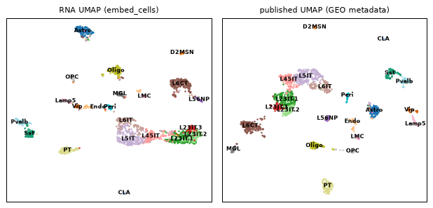
embed_cells(cd, source="rna") selects the numeric rna.* columns. Count features are normalised with normalize_counts; library_size=True suits transcriptome-wide data. The function then runs PCA on the normalised matrix, and t-SNE and UMAP on the PCs. The results are cd.cellm["rna_pca"], ["rna_tsne"] and ["rna_umap"], with rows in the order of cd.cells. The parameters go to cd.uns["embeddings"].

t = time.time()
out = emb.embed_cells(cd, source="rna", library_size=True, n_pcs=30)
print({k: v.shape for k, v in out.items()}, f"in {time.time() - t:.0f} s")
meta = cd.uns["embeddings"]["rna_pca"]
print(meta["normalization"], "|", meta["n_features"], "features | variance of PC1-5:",
      np.round(meta["explained_variance_ratio"][:5], 3))

fig, axes = plt.subplots(1, 2, figsize=(7, 3.4))
scatter(axes[0], cd.cellm["rna_umap"], y_type, "RNA UMAP (embed_cells)")
scatter(axes[1], cd.cellm["paper_umap"], y_type, "published UMAP (GEO metadata)")
fig.tight_layout()

{'rna_pca': (2000, 30), 'rna_tsne': (2000, 2), 'rna_umap': (2000, 2)} in 9 s
library-size (median total), log1p, z-score per feature | 2000 features | variance of PC1-5: [0.05  0.029 0.026 0.021 0.018]

4. cluster_cells: Leiden clusters and agreement with the published cell types

cluster_cells builds a k-nearest-neighbour graph (k = 15) on an embedding and partitions it with the Leiden algorithm. The labels are stored as a categorical column of cd.cells and the parameters in cd.uns["clusters"]. We compare them with the 22 published cell types and with the three coarse classes, using the adjusted Rand index (ARI; 0 = chance, 1 = identical) and normalised mutual information (NMI).

lab_rna = emb.cluster_cells(cd, use="rna_pca", resolution=1.0, key_added="leiden_rna")
print(f"{lab_rna.nunique()} RNA clusters;", "vs cell types", agreement(lab_rna, y_type),
      "| vs coarse classes", agreement(lab_rna, y_class))

# each cluster: size, its most frequent published type and that type's share
tab = pd.crosstab(lab_rna, cd.cells["cell_type"])
summary = pd.DataFrame({"n_cells": tab.sum(axis=1), "main_type": tab.idxmax(axis=1),
                        "share": (tab.max(axis=1) / tab.sum(axis=1)).round(2)})
summary.T

17 RNA clusters; vs cell types {'ARI': 0.675, 'NMI': 0.804} | vs coarse classes {'ARI': 0.144, 'NMI': 0.414}

leiden_rna	0	1	2	3	4	5	6	7	8	9	10	11	12	13	14	15	16
n_cells	256	222	205	173	163	160	116	115	108	95	79	74	60	54	49	37	34
main_type	L23IT.1	L6IT	L6CT	L5IT	L23IT.2	Astro	Oligo	PT	L45IT	Lamp5	Pvalb	Sst	D2MSN	MGL	OPC	Peri	L56NP
share	0.71	0.57	0.99	0.92	0.43	0.91	0.92	0.98	0.94	0.43	0.92	0.99	0.4	0.83	0.92	0.89	0.94

Most clusters map to one published type: more than 80 % of their cells share it. The exceptions are the L2/3 IT subgroups, L6 IT and two small interneuron groups (Lamp5, D2MSN), which the clusters of 2,000 cells at resolution 1 mix with their neighbours. The published labels come from a finer analysis of the full transcriptome of all cells. So the ARI is well below 1, while the NMI stays high.

5. marker_features: what distinguishes each group

marker_features ranks the prefix columns of cd.cells by the difference of the mean of log1p(value) between a group and all other cells. Applied to the published types, it recovers known markers:

• Plp1 / Mobp / St18 in oligodendrocytes and Ptprz1 in OPCs;

• Slc1a2 / Slc1a3 in astrocytes and Inpp5d / Dock2 in microglia;

• Kcnc2 in Pvalb interneurons;

• Foxp2 in L6 corticothalamic neurons and Tshz2 in L5/6 near-projecting neurons.

Applied to the Leiden clusters, it describes clusters that have no label yet; for example, Cux2 comes out for the L2/3 IT cluster.

by_type = emb.marker_features(cd, "cell_type", prefix="rna.", n_top=4)
show = ["Oligo", "OPC", "Astro", "MGL", "Endo", "Peri", "Pvalb", "Sst", "Vip", "L6CT", "PT", "L56NP"]
display(pd.DataFrame({t: by_type[t] for t in show}).rename_axis("rank"))

by_cluster = emb.marker_features(cd, "leiden_rna", prefix="rna.", n_top=4)
pd.DataFrame({f"{c} ({summary.loc[c, 'main_type']})": by_cluster[c] for c in summary.index[:8]}).rename_axis("rank")

	Oligo	OPC	Astro	MGL	Endo	Peri	Pvalb	Sst	Vip	L6CT	PT	L56NP
rank
0	Plp1	Lhfpl3	Gpc5	Tgfbr1	Bnc2	Flt1	Erbb4	Nxph1	Adarb2	Hs3st4	Tafa1	Tshz2
1	St18	Sox2ot	Slc1a2	Inpp5d	Fbxl7	Slco1a4	Nxph1	Grik1	Erbb4	Foxp2	Gm2164	Vwc2l
2	Mobp	Nxph1	Slc1a3	Lrmda	Eya2	Ebf1	Kcnc2	Synpr	Npas3	Zfpm2	Pex5l	Nxph1
3	Mbp	Ptprz1	Mertk	Dock2	Nxn	Mecom	Btbd11	Npas3	Zfp536	Grik3	Tcerg1l	Olfm3

	0 (L23IT.1)	1 (L6IT)	2 (L6CT)	3 (L5IT)	4 (L23IT.2)	5 (Astro)	6 (Oligo)	7 (PT)
rank
0	Cux2	Galnt14	Hs3st4	Pcdh15	Epha6	Gpc5	Plp1	Tafa1
1	Lingo2	Sorcs3	Foxp2	Cpne4	Slit3	Slc1a2	St18	Gm2164
2	Rasgrf2	Il1rapl2	Zfpm2	Cntn5	March1	Mertk	Mbp	Pex5l
3	Unc5d	Grik3	Grik3	Zfp804b	Grm1	Slc1a3	Mobp	Tcerg1l

6. Contact maps: scHiCluster features from the linked .scool

The same nuclei also have a contact map. scool_cell_features computes the features of scHiCluster (Zhou et al. 2019, PNAS) as follows:

1. Read the 1 Mb intra-chromosomal map of each chromosome of each cell from the .scool.

2. Smooth it with a 3 × 3 convolution.

3. Impute it by random walk with restart (uchrom.emb.hic.schicluster_impute).

4. Keep the top 20 % of the entries (set them to 1, the rest to 0).

5. Reduce each chromosome to 20 PCs across cells, and concatenate the PCs of all chromosomes.

The per-cell maps are embedded in the atlas store, partitioned by chromosome with the cells in order (embedded/contacts/per_cell; layout in packages/chromdata/spec.md). load_linked_scool(key="per_cell", cell=...) exports one cell to a cooler file on demand; for many cells, chromdata.embedded.export_scool reads each chromosome’s partition once for all of them. We write the intra-chromosomal maps of the 2,000 cells (all that scHiCluster uses: trans=False) as a local .scool in _out/; scool_cell_features and the web browser read that file.

import cooler
from chromdata.embedded import export_scool

URL = ds.list_atlas().loc["schicar_mouse_cortex", "url"]          # where the store is
t = time.time()
export_scool(URL, "per_cell", SCOOL, cells=cd.cells.index, trans=False)
print(f"{SCOOL}: {len(cooler.fileops.list_scool_cells(str(SCOOL))):,} cells, "
      f"{SCOOL.stat().st_size / 1e6:.0f} MB, in {time.time() - t:.0f} s")

_out/schicar_mop_2000_cells_1Mb.scool: 2,000 cells, 80 MB, in 22 s

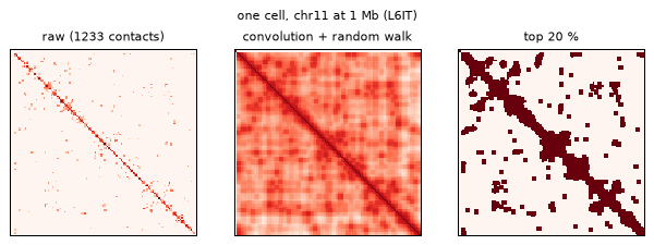
First, look at one cell. Its chr11 map from the local file is the same as the one load_linked_scool exports from the atlas store. The raw map is very sparse, and imputation spreads its contacts along the diagonal and into domains.

from uchrom.emb.hic import schicluster_impute

cell = cd.cells["n_contacts_hic"].sort_values().index[int(0.75 * cd.n_cells)]   # a cell at the 75th depth percentile
raw = cooler.Cooler(f"{SCOOL}::/cells/{cell}").matrix(balance=False).fetch("chr11").astype(float)
one = full.load_linked_scool(key="per_cell", cell=cell)          # the store's own export of this cell
print("same chr11 map as load_linked_scool:", np.array_equal(raw, one.matrix(balance=False).fetch("chr11")))
imputed = schicluster_impute(raw, pad=1, rp=0.5)
iu = np.triu_indices_from(imputed, 1)
binary = imputed > np.percentile(imputed[iu], 80)

fig, axes = plt.subplots(1, 3, figsize=(7, 2.5))
for ax, m, title in zip(axes, [np.log1p(raw), np.log(np.maximum(imputed, 1e-6)), binary],
                        [f"raw ({int(np.triu(raw).sum())} contacts)", "convolution + random walk", "top 20 %"]):
    ax.imshow(m, cmap="Reds", interpolation="none")
    ax.set_title(title, fontsize=9); ax.set_xticks([]); ax.set_yticks([])
fig.suptitle(f"one cell, chr11 at 1 Mb ({cd.cells.loc[cell, 'cell_type']})", fontsize=9)
fig.tight_layout()

same chr11 map as load_linked_scool: True

Now compute the features of all 2,000 cells (about a minute) and embed them. The features are already reduced and scaled, so embed_cells gets them as a matrix= with normalization="none". The features= text is recorded with the embedding.

CHROMS = [f"chr{i}" for i in range(1, 20)] + ["chrX"]
t = time.time()
feats, cols, depth = emb.scool_cell_features(str(SCOOL), [str(c) for c in cd.cells.index], chroms=CHROMS)
print(f"scHiCluster features {feats.shape} in {time.time() - t:.0f} s; e.g. {cols[:3]}")
n_all = cd.cells["n_contacts_hic"].to_numpy()                     # all contacts per cell (stored)
assert (depth <= n_all).all()                                    # the scool holds the intra-chromosomal ones
print(f"{depth.sum():,} intra-chromosomal contacts ({depth.sum() / n_all.sum():.0%} of all)")

emb.embed_cells(cd, source="hic", matrix=feats, normalization="none", n_pcs=20,
                features="scHiCluster: 1 Mb maps chr1-19, X; 3x3 convolution, random walk (rp=0.5), "
                         "top 20% binarised, 20 PCs per chromosome")
r_depth = [round(float(np.corrcoef(cd.cellm["hic_pca"][:, j], np.log(n_all))[0, 1]), 2) for j in range(3)]
print("Pearson r of Hi-C PC1-3 with log(contacts):", r_depth)

lab_hic = emb.cluster_cells(cd, use="hic_pca", resolution=1.0, key_added="leiden_hic")
lab_hic2 = emb.cluster_cells(cd, use="hic_pca", resolution=0.3, key_added="leiden_hic_coarse")
print(f"{lab_hic.nunique()} Hi-C clusters (resolution 1):", "vs cell types", agreement(lab_hic, y_type))
print(f"{lab_hic2.nunique()} Hi-C clusters (resolution 0.3):", "vs coarse classes", agreement(lab_hic2, y_class))
pd.crosstab(lab_hic2, cd.cells["cell_class"]).rename_axis(index="leiden_hic_coarse", columns=None)

scHiCluster features (2000, 400) in 34 s; e.g. ['chr1_PC1', 'chr1_PC2', 'chr1_PC3']
33,850,441 intra-chromosomal contacts (74% of all)

Pearson r of Hi-C PC1-3 with log(contacts): [-0.23, 0.57, -0.04]

6 Hi-C clusters (resolution 1): vs cell types {'ARI': 0.11, 'NMI': 0.243}
2 Hi-C clusters (resolution 0.3): vs coarse classes {'ARI': 0.573, 'NMI': 0.53}

	excitatory	inhibitory	non-neuronal
leiden_hic_coarse
0	1272	233	35
1	33	14	413

CLASS_COLORS = {"excitatory": "tab:red", "inhibitory": "tab:blue", "non-neuronal": "tab:green"}
fig, axes = plt.subplots(1, 2, figsize=(7, 3.4))
scatter(axes[0], cd.cellm["hic_umap"], y_class, "Hi-C UMAP: coarse class", palette=CLASS_COLORS, annotate=False)
axes[0].legend(fontsize=7, markerscale=3, frameon=False, loc="best")
xy = cd.cellm["hic_umap"]
sc = axes[1].scatter(xy[:, 0], xy[:, 1], s=4, lw=0, c=np.log10(cd.cells["n_contacts_hic"]), cmap="viridis")
fig.colorbar(sc, ax=axes[1], label="log10 contacts per cell")
axes[1].set_title("Hi-C UMAP: sequencing depth", fontsize=9); axes[1].set_xticks([]); axes[1].set_yticks([])
fig.tight_layout()

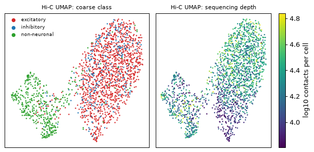
At 1 Mb, single-cell contact maps separate neurons from non-neuronal cells, but not the finer neuronal subtypes. The fine-type ARI is therefore much lower than for RNA. Within the neurons, the main gradient follows the number of contacts per cell: PC2 tracks sequencing depth (r above).

7. Sparse counts: tfidf_lsi and the agreement of the modalities

For sparse counts such as ATAC fragments, embed_cells(..., normalization="tfidf") (the default for source="atac") calls tfidf_lsi: TF-IDF, then truncated SVD (latent semantic indexing). Component 1 is dropped when it tracks sequencing depth. The store’s atac.* columns count fragments in the gene body + 2 kb of 484 genes, and they show the depth effect clearly. These windows hold few fragments per cell, so the build recipe used 100 kb genome bins for the stored atac_lsi instead.

gact = full.cells.iloc[keep][[c for c in full.cells.columns if c.startswith("atac.")]].to_numpy()
lsi, info = emb.tfidf_lsi(gact, n_components=30)
print(f"gene-activity counts: median {np.median(gact.sum(1)):.0f} fragments per cell in {gact.shape[1]} genes")
print("r(LSI component, log depth) for components 1-3:", np.round(info["depth_r"][:3], 2),
      "-> dropped", info["dropped"])
print("kNN-10 purity: gene-activity LSI", knn_purity(lsi, y_type),
      "| stored atac_lsi (100 kb bins)", knn_purity(cd.cellm["atac_lsi"], y_type))

gene-activity counts: median 630 fragments per cell in 484 genes
r(LSI component, log depth) for components 1-3: [ 0.98 -0.76 -0.13] -> dropped [1]
kNN-10 purity: gene-activity LSI 0.104 | stored atac_lsi (100 kb bins) 0.298

The same cells, four views. Leiden clusters are computed at resolution 1 on each linear embedding and compared with the 22 types. The kNN purity is measured in the embedding itself, for the 22 types and for the 3 classes. Its chance level is the purity after shuffling the labels; it is printed first.

lab_atac = emb.cluster_cells(cd, use="atac_lsi", resolution=1.0, key_added="leiden_atac")
rows = []
for key, lab in [("rna_pca", lab_rna), ("atac_lsi", lab_atac), ("hic_pca", lab_hic), ("paper_umap", None)]:
    x = cd.cellm[key]
    row = {"embedding": key, "modality": cd.uns["embeddings"][key]["modality"], "dims": x.shape[1],
           "kNN purity (type)": knn_purity(x, y_type), "kNN purity (class)": knn_purity(x, y_class)}
    if lab is not None:
        row.update({"clusters": lab.nunique(), "ARI type": agreement(lab, y_type)["ARI"],
                    "NMI type": agreement(lab, y_type)["NMI"]})
    rows.append(row)
rng = np.random.default_rng(1)
print("chance purity:", knn_purity(cd.cellm["rna_pca"], rng.permutation(y_type)),
      "(type),", knn_purity(cd.cellm["rna_pca"], rng.permutation(y_class)), "(class)")
print("ARI between RNA and Hi-C clusters:", round(adjusted_rand_score(lab_rna, lab_hic), 3),
      "| RNA and ATAC clusters:", round(adjusted_rand_score(lab_rna, lab_atac), 3))
pd.DataFrame(rows).set_index("embedding")

chance purity: 0.07 (type), 0.489 (class)
ARI between RNA and Hi-C clusters: 0.118 | RNA and ATAC clusters: 0.251

	modality	dims	kNN purity (type)	kNN purity (class)	clusters	ARI type	NMI type
embedding
rna_pca	RNA	30	0.859	0.972	17.0	0.675	0.804
atac_lsi	ATAC	30	0.298	0.826	7.0	0.226	0.382
hic_pca	Hi-C	20	0.235	0.761	6.0	0.110	0.243
paper_umap	Published	2	0.934	0.979	NaN	NaN	NaN

8. Imaging: IF signals summarised per cell (aggregate_tracks)

DNA seqFISH+ in the Takei 2025 cerebellum measured 48 IF channels at every DNA spot (histone marks, nuclear bodies, chromatin proteins); they are stored as spot_tracks. aggregate_tracks turns per-spot tracks into per-cell features:

• stat="mean" gives one mean per channel (if.<mark>), useful for colouring;

• stat="corr" gives the within-cell Pearson correlation of every pair of channels over the cell’s spots (1,128 pairs). This describes which marks occur together on the same loci and does not depend on each cell’s overall staining intensity.

The atlas store has 10.9 M spots. ds.atlas opens it backed over HTTP, and iter_cells streams it in batches of 64 cells, reading the coordinates and only the 48 IF tracks (about 1.5 min; the store’s other spot tracks are not fetched).

from uchrom.io.seqfish_multiomics import IF_COLUMNS

t = time.time()
takei = ds.atlas("takei2025_cerebellum")                  # backed, over HTTP
marks = [c for c in IF_COLUMNS if c in takei.spot_tracks.columns]
print(f"{takei.n_cells:,} cells, {takei.n_spots:,} spots, {len(marks)} IF channels, e.g. {marks[:6]}")

corr, means = [], []
for chunk in takei.iter_cells(batch=64, columns="coords", tracks=marks):
    corr.append(emb.aggregate_tracks(chunk, marks, prefix="if", stat="corr", write=False))
    means.append(emb.aggregate_tracks(chunk, marks, prefix="if", stat="mean", write=False))
order = takei.cells.index.astype(str)
corr = pd.concat(corr).reindex(order)
means = pd.concat(means).reindex(order).set_axis(takei.cells.index)
takei.cells = pd.concat([takei.cells, means], axis=1)        # if.<mark> means as cell columns
print(f"per-cell features: corr {corr.shape}, means {means.shape} in {time.time() - t:.0f} s")

emb.embed_cells(takei, source="if", matrix=corr.to_numpy(), normalization="zscore", n_pcs=20,
                features="within-cell Pearson r of 48 IF channels over all spots (1,128 pairs)")
y_cb = takei.cells["cell_type"].astype(str).to_numpy()
lab_if = emb.cluster_cells(takei, use="if_pca", resolution=0.3, key_added="leiden_if")
print(f"{lab_if.nunique()} IF clusters:", agreement(lab_if, y_cb),
      "| kNN-10 purity", knn_purity(takei.cellm["if_pca"], y_cb),
      "(chance", knn_purity(takei.cellm["if_pca"], np.random.default_rng(1).permutation(y_cb)), ")")
z_means = ((means - means.mean()) / means.std()).to_numpy()   # the means are z-scores already; rescale per mark
print("with per-cell means instead of correlations: kNN-10 purity",
      knn_purity(PCA(20, random_state=0).fit_transform(z_means), y_cb))
pd.crosstab(lab_if, takei.cells["cell_type"]).rename_axis(index="leiden_if", columns=None)

1,799 cells, 10,912,638 spots, 48 IF channels, e.g. ['CPSF6', 'ATRX', 'H4K8ac', 'HDAC2', 'H3K9ac', 'H3K9me3']

per-cell features: corr (1799, 1128), means (1799, 48) in 91 s

4 IF clusters: {'ARI': 0.299, 'NMI': 0.386} | kNN-10 purity 0.737 (chance 0.426 )
with per-cell means instead of correlations: kNN-10 purity 0.667

	Bergmann	Granule	MLI1	MLI2+PLI	Other	Purkinje
leiden_if
0	9	650	0	3	161	3
1	21	452	5	0	107	2
2	160	6	4	1	46	3
3	2	1	81	23	9	50

fig, axes = plt.subplots(1, 2, figsize=(7, 3.4))
scatter(axes[0], takei.cellm["if_umap"], y_cb, "IF correlation UMAP")
scatter(axes[1], takei.cellm["if_umap"], lab_if.astype(str).radd("c"), "IF Leiden clusters", annotate=True)
fig.tight_layout()

top = emb.marker_features(takei, "cell_type", prefix="if.", n_top=3, log=False)   # IF values are z-scores
pd.DataFrame(top).rename_axis("rank")

	Granule	Bergmann	Other	MLI1	Purkinje	MLI2+PLI
rank
0	RING1B	H3K9ac	LaminB1	mH2A1	H3K27me3	mH2A1
1	H3	SOX2	SUZ12	H3K9ac	H4K8ac	H3K9me3
2	SUZ12	H3K27ac	SF3A66	H3K27ac	H3K9ac	H3K9ac

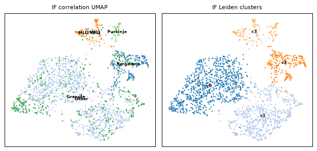
The IF correlation embedding groups the cerebellar types well above chance, and better than the per-cell means. The Leiden clusters give:

• one cluster of Bergmann glia;

• one cluster of the molecular-layer interneurons (MLI1, MLI2+PLI) together with the Purkinje cells;

• two clusters that both mix granule cells with the heterogeneous “Other” group.

So the ARI stays modest. The published types were derived from the transcriptome, so they are a demanding reference for chromatin marks alone. Among the per-cell means, SOX2 comes out for Bergmann glia, which express it.

9. How embeddings are stored

• cd.cellm[key]: one array per embedding, with rows aligned with cd.cells (rna_pca, rna_umap, hic_pca, …).

• cd.uns["embeddings"][key]: what embed_cells recorded. This includes source, modality, method, label and axis_prefix, plus the normalisation, the number of features and their names, and the explained variance. The web browser groups its Embedding view by modality and labels the axes with axis_prefix.

• cd.uns["clusters"][key]: the Leiden parameters. The labels themselves are categorical cd.cells columns, which the browser offers as colourings, like cell_type.

All of this round-trips through a .chromdata.zarr store. The .scool written in section 6 stays linked: its relative path resolves against the folder of the store.

pd.DataFrame(cd.uns["embeddings"]).T[["source", "modality", "method", "label", "axis_prefix", "n_features"]]

	source	modality	method	label	axis_prefix	n_features
paper_umap	GSE305439 metadata	Published	umap	Paper UMAP (RNA)	UMAP	NaN
atac_lsi	atac	ATAC	lsi	ATAC LSI	LSI	25461
rna_pca	rna	RNA	pca	RNA PCA	PC	2000
rna_tsne	rna	RNA	tsne	RNA t-SNE	tSNE	2000
rna_umap	rna	RNA	umap	RNA UMAP	UMAP	2000
hic_pca	hic	Hi-C	pca	Hi-C PCA	PC	400
hic_tsne	hic	Hi-C	tsne	Hi-C t-SNE	tSNE	400
hic_umap	hic	Hi-C	umap	Hi-C UMAP	UMAP	400

path = OUT / "schicar_mop_2000_embeddings.chromdata.zarr"
cd.write(path)
back = ChromData.read(path)
same = all(np.allclose(back.cellm[k], cd.cellm[k]) for k in cd.cellm)
print(path, "| cellm keys:", sorted(back.cellm), "| arrays equal:", same)
print("clusters:", {k: v["n_clusters"] for k, v in back.uns["clusters"].items()},
      "| link problems:", back.validate_links())

# what the web browser lists for this store (the same call its /api/datasets endpoint makes)
from uchrom_browser.data import DatasetStore

store = DatasetStore().load(str(path))
pd.DataFrame(store.embeddings())

_out/schicar_mop_2000_embeddings.chromdata.zarr | cellm keys: ['atac_lsi', 'hic_pca', 'hic_tsne', 'hic_umap', 'paper_umap', 'rna_pca', 'rna_tsne', 'rna_umap'] | arrays equal: True
clusters: {'leiden_rna': 17, 'leiden_hic': 6, 'leiden_hic_coarse': 2, 'leiden_atac': 7} | link problems: []

	key	method	source	modality	label	n_dims
0	paper_umap	umap	GSE305439 metadata	Published	Paper UMAP (RNA)	2
1	atac_lsi	lsi	atac	ATAC	ATAC LSI	30
2	rna_pca	pca	rna	RNA	RNA PCA	30
3	rna_tsne	tsne	rna	RNA	RNA t-SNE	2
4	rna_umap	umap	rna	RNA	RNA UMAP	2
5	hic_pca	pca	hic	Hi-C	Hi-C PCA	20
6	hic_tsne	tsne	hic	Hi-C	Hi-C t-SNE	2
7	hic_umap	umap	hic	Hi-C	Hi-C UMAP	2

To look at the store interactively, run python -m uchrom_browser tutorials/_out/schicar_mop_2000_embeddings.chromdata.zarr. The Embedding view lists the arrays above, grouped by modality, and can colour cells by cell_type, the Leiden columns or any rna.<gene>. The linked .scool shows the (intra-chromosomal) contact maps of a selected cell.

print(f"total runtime {time.time() - T0:.0f} s")

total runtime 178 s

Next steps

• higashi_embedding.ipynb: a contact-map embedding with FastHigashi (tensor decomposition) instead of scHiCluster, on sci-Hi-C of two cell lines.

• plotting_and_browser.ipynb: the web browser (uchrom_browser), which shows the embeddings stored here.

• chromdata_basics.ipynb and chromdata_stores.ipynb: the ChromData container (cells, cellm, uns, linked files) and its .chromdata.zarr store, including backed reading as used for the Takei data.

• import_seqfish_multiomics.ipynb: the Takei 2025 seqFISH+ data: traces, IF tracks and cell types.