Spot-to-trace alignment with jie

Multiplexed DNA-FISH first gives detections: spots with a decoded locus and a 3-D position, but no link between the spots of one chromosome copy. A cell typically has 1–7 candidate spots per locus (two homologs, sister chromatids after replication, false detections), and some loci are missed. uchrom.im.trace.align_spots decides which spots form one chromatin fibre: it is an independent re-implementation of jie (Jia & Ren 2022, Nature Biotechnology, doi:10.1038/s41587-022-01568-9). For each (cell, chromosome) it builds a graph over the candidate spots ordered along the genome, scores each link by a Gaussian-chain polymer model (how plausible is this 3-D distance for this genomic distance?), extracts the best path as one fibre, masks its spots and repeats — so the number of copies (ploidy) comes out of the data — and finally groups fibres that stay close as sister chromatids.

Data: Takei et al. 2021, Nature 590:344 — raw DNA seqFISH+ detections of E14 mouse ES cells at 25 kb (Zenodo 3735329, DNAseqFISH+.zip, 144 MB, downloaded once by ds.fetch("seqfish"); replicate 1: 201 cells, 20 chromosomes × 60 loci, 316,995 spots). The same experiment’s traced table is the 4DN FOF-CT file 4DNFIHF3JCBY (ds.fetch("takei"), 22 MB; see import_fofct.ipynb), which we use for the genomic coordinates and as the reference assignment. Runtime: about a minute (all chromosomes).

from pathlib import Path
import time
import zipfile

import numpy as np
import pandas as pd
import matplotlib.pyplot as plt
from sklearn.metrics import adjusted_rand_score
from chromdata import ChromData
from uchrom.im.trace import align_spots, SpotAlignerParams
import uchrom.datasets as ds
import uchrom.fea as fea

plt.rcParams["figure.dpi"] = 90

OUT = Path("_out"); OUT.mkdir(exist_ok=True)   # outputs: tutorials/_out/ (ignored by git)

SEQFISH_ZIP = ds.fetch("seqfish")   # raw seqFISH+ detections (Zenodo 3735329, 144 MB; downloaded once)
FOFCT = ds.fetch("takei")           # the traced FOF-CT core table of the same experiment (4DN, 22 MB)
for p in (SEQFISH_ZIP, FOFCT):
    print(f"{p.relative_to(ds.data_dir())}  ({p.stat().st_size / 1e6:.0f} MB)")

DNAseqFISH+.zip  (144 MB)
4DNFIHF3JCBY.csv  (22 MB)

1. The raw detections

The zip holds eight tables (1 Mb and 25 kb loci, several replicates); we read the 25-kb replicate 1 directly from it. Columns: fov, cellID (numbered within each FOV), the locus index regionID (hyb1-60), chromID (1–19, 20 = X), x, y in 103-nm pixels and z in 250-nm steps, intensities, and labelID — the upstream pipeline’s homolog call (0, 1; rarely 2, 3; −1 = rejected). We keep labelID aside as the reference and never show it to the aligner.

with zipfile.ZipFile(SEQFISH_ZIP) as zf, zf.open("DNAseqFISH+/DNAseqFISH+25kbloci-E14-replicate1.csv") as fh:
    raw = pd.read_csv(fh)
raw["cell_id"] = raw["fov"].astype(str) + "_" + raw["cellID"].astype(str)   # cellID repeats across FOVs
raw["chrom"] = raw["chromID"].map(lambda c: "chrX" if c == 20 else f"chr{c}")

per_locus = raw.groupby(["cell_id", "chrom", "regionID (hyb1-60)"]).size()
print(f"{len(raw):,} detections, {raw['cell_id'].nunique()} cells in {raw['fov'].nunique()} FOVs, "
      f"{raw['chrom'].nunique()} chromosomes x {raw['regionID (hyb1-60)'].nunique()} loci")
print("candidate spots per (cell, chromosome, locus):", per_locus.value_counts().sort_index().to_dict())
print("upstream labelID:", raw["labelID"].value_counts().sort_index().to_dict())
raw[["fov", "cellID", "chromID", "regionID (hyb1-60)", "x", "y", "z", "dot_intensity", "labelID"]].head()

316,995 detections, 201 cells in 5 FOVs, 20 chromosomes x 60 loci
candidate spots per (cell, chromosome, locus): {1: 93313, 2: 77662, 3: 18664, 4: 2740, 5: 251, 6: 24, 7: 1}
upstream labelID: {-1: 2487, 0: 171962, 1: 140231, 2: 2240, 3: 75}

	fov	cellID	chromID	regionID (hyb1-60)	x	y	z	dot_intensity	labelID
0	0	1	1	2	1718.431196	146.909289	11.282036	638	0
1	0	1	1	3	1717.986519	146.171951	11.083011	738	0
2	0	1	1	3	1604.490932	204.195855	11.725510	223	1
3	0	1	1	5	1718.106776	146.904642	10.363083	775	0
4	0	1	1	5	1600.751787	204.916308	13.133202	787	1

The 4DN FOF-CT table 4DNFIHF3JCBY deposits exactly these detections after tracing: matching the spots by position (pixels × voxel size = µm, 3 decimals) shows the same cell ids, the trace suffix equal to labelID, and gives each (chromosome, regionID) its mm10 locus.

fofct = ChromData.from_fofct(FOFCT).to_dataframe()
key = lambda x, y, z: pd.MultiIndex.from_arrays([np.round(x, 3), np.round(y, 3), np.round(z, 3)])
f_idx = pd.Series(np.arange(len(fofct)), index=key(fofct["x"], fofct["y"], fofct["z"]))
row = f_idx.reindex(key(raw["x"] * 0.103, raw["y"] * 0.103, raw["z"] * 0.25)).to_numpy()
matched = fofct.iloc[row]
print(f"matched {np.isfinite(row).sum():,} of {len(raw):,} detections; same cell "
      f"{np.mean(matched['cell_id'].astype(str).to_numpy() == raw['cell_id'].to_numpy()):.1%}, "
      f"trace suffix == labelID "
      f"{np.mean(matched['trace_id'].astype(str).str.rsplit('_', n=1).str[-1].to_numpy() == raw['labelID'].astype(str).to_numpy()):.1%}")

locus = (pd.DataFrame({"chrom": raw["chrom"], "region": raw["regionID (hyb1-60)"],
                       "start": matched["start"].to_numpy(), "end": matched["end"].to_numpy()})
         .drop_duplicates(["chrom", "region"]).set_index(["chrom", "region"]))
print(f"{len(locus)} (chromosome, regionID) -> mm10 loci, e.g.", locus.iloc[0].to_dict())

matched 316,995 of 316,995 detections; same cell 100.0%, trace suffix == labelID 100.0%
1200 (chromosome, regionID) -> mm10 loci, e.g. {'start': 135625000, 'end': 135650000}

2. The align_spots input

align_spots takes one row per detection: cell_id, chrom, start, end, x, y, z in nm (optional sigma_x/y/z localisation errors and a spot_id carried through). Several rows may share a (cell, locus) — resolving them is the job.

xyz_nm = np.column_stack([raw["x"] * 103.0, raw["y"] * 103.0, raw["z"] * 250.0])
loci = locus.loc[list(zip(raw["chrom"], raw["regionID (hyb1-60)"]))]
spots_df = pd.DataFrame({
    "spot_id": np.arange(len(raw)),
    "cell_id": raw["cell_id"].to_numpy(),
    "chrom": raw["chrom"].to_numpy(),
    "start": loci["start"].to_numpy(), "end": loci["end"].to_numpy(),
    "x": xyz_nm[:, 0], "y": xyz_nm[:, 1], "z": xyz_nm[:, 2],
})
label = raw["labelID"].to_numpy()          # reference only
spots_df.head()

	spot_id	cell_id	chrom	start	end	x	y	z
0	0	0_1	chr1	135625000	135650000	176998.413188	15131.656798	2820.508940
1	1	0_1	chr1	135650000	135675000	176952.611457	15055.710912	2770.752832
2	2	0_1	chr1	135650000	135675000	165262.565996	21032.173096	2931.377597
3	3	0_1	chr1	135700000	135725000	176964.997928	15131.178147	2590.770663
4	4	0_1	chr1	135700000	135725000	164877.434061	21106.379765	3283.300545

3. One chromosome first: what the parameters do

On chr19 (15,000 detections in 201 cells) compare the defaults with settings suited to this data, scoring each run against labelID (only spots with labelID ≥ 0):

• assigned — fraction of labelled spots placed on some fibre;

• purity — per called fibre, the fraction of its spots from its majority labelID;

• ARI — per cell, adjusted Rand index between fibres and labelID (median over cells).

The default max_skip=3 lets a path jump over at most 3 undetected loci; with ~35 % of loci missed per copy, paths break and most spots stay unassigned. Allowing longer skips (max_skip=12) with a larger per-skip penalty, at least 10 spots per fibre, at most 4 fibres per (cell, chromosome), and rejecting paths whose mean link cost exceeds 8 assigns most spots. We chose these on chr19 by this comparison — a calibration against the reference, so the genome-wide run below is the fairer test. The scale factor τ (nm per bp) is fitted per chromosome from the data unless you pass tau_by_chrom.

def score(cd, ref_spots, ref_label):
    """Compare called fibres with the reference labels (spots with label >= 0)."""
    called = pd.Series(cd.spots["trace_id"].astype(str).to_numpy(), index=cd.spots["spot_id"].to_numpy())
    fibre = called.reindex(ref_spots["spot_id"].to_numpy()).to_numpy()
    df = pd.DataFrame({"cell": ref_spots["cell_id"].to_numpy(), "chrom": ref_spots["chrom"].to_numpy(),
                       "fibre": fibre, "label": ref_label})
    df = df[df["label"] >= 0]
    on = df[pd.notna(df["fibre"])]
    purity = on.groupby("fibre")["label"].agg(lambda s: s.value_counts().iloc[0] / len(s))
    ari = [adjusted_rand_score(g["label"], g["fibre"].fillna("none"))
           for _, g in df.groupby(["cell", "chrom"]) if g["label"].nunique() > 1]
    return pd.Series({"assigned": pd.notna(df["fibre"]).mean(), "purity": purity.mean(),
                      "median ARI": np.median(ari) if ari else np.nan})


chr19 = (spots_df["chrom"] == "chr19").to_numpy()
TUNED = SpotAlignerParams(max_skip=12, gap_penalty=5.0, min_spots_per_fiber=10, max_fibers_per_chrom=4,
                          mean_edge_weight_cutoff=8.0, sister_pair_radius_nm=400.0)
rows = {}
for name, params in [("defaults", SpotAlignerParams()), ("tuned", TUNED)]:
    t0 = time.perf_counter()
    res = align_spots(spots_df[chr19], params=params)
    rows[name] = score(res, spots_df[chr19], label[chr19])
    rows[name]["fibres per (cell, chr)"] = res.results["ploidy"]["n_fibers"].mean()
    rows[name]["seconds"] = time.perf_counter() - t0
print("fitted tau:", {c: round(v["tau_nm_per_bp"], 4) for c, v in res.uns["jie_polymer"].items()}, "nm/bp")
pd.DataFrame(rows).round(3)

fitted tau: {'chr19': 0.0074} nm/bp

	defaults	tuned
assigned	0.576	0.828
purity	0.863	0.977
median ARI	0.424	0.721
fibres per (cell, chr)	1.254	1.856
seconds	2.008	3.075

4. All chromosomes

The aligner works per (cell, chromosome), so the genome-wide run is the same call on all detections (~4,000 graphs). It returns a ChromData: spots (the kept detections with their trace_id, spot_id carried through), traces (one row per fibre: cell, chromosome, number of spots, path cost, sister group), results['ploidy'] (fibres and sister groups per (cell, chromosome)) and uns['jie_polymer'] (the fitted τ per chromosome).

t0 = time.perf_counter()
cd = align_spots(spots_df, params=TUNED)
print(f"aligned in {time.perf_counter() - t0:.0f} s\n")
print(cd)
cd.traces.head()

aligned in 62 s

ChromData: n_spots=270451, n_traces=7515, n_cells=201, n_bins=1200
  spots:   ['chrom', 'start', 'end', 'trace_id', 'cell_id', 'spot_id', 'bin_id']
  traces:  ['trace_id', 'cell_id', 'chrom', 'n_spots', 'path_weight', 'mean_edge', 'sister_group'] (7515 traces)
  results: ['ploidy']
  uns:     ['jie_polymer', 'jie_params']

	trace_id	cell_id	chrom	n_spots	path_weight	mean_edge	sister_group
0	0	0_1	chr1	37	100.762165	2.651636	0
1	1	0_1	chr1	32	122.095657	3.699868	1
2	2	0_1	chr10	39	94.118443	2.352961	2
3	3	0_1	chr10	37	113.078246	2.975743	3
4	4	0_1	chr11	33	69.845648	2.054284	4

ploidy = cd.results["ploidy"]
per_chrom = {}
for chrom in sorted(cd.spots["chrom"].astype(str).unique(), key=lambda c: (c == "chrX", len(c), c)):
    m = (spots_df["chrom"] == chrom).to_numpy()
    s = score(cd.get_chrom(chrom), spots_df[m], label[m])
    s["2 fibres"] = (ploidy.loc[ploidy["chrom"] == chrom, "n_fibers"] == 2).mean()
    per_chrom[chrom] = s
per_chrom = pd.DataFrame(per_chrom).T
auto = per_chrom.drop(index="chrX")
print(f"autosomes: {auto['assigned'].mean():.1%} of labelled spots assigned, purity {auto['purity'].mean():.3f}, "
      f"median ARI {auto['median ARI'].mean():.2f}, two fibres in {auto['2 fibres'].mean():.0%} of (cell, chromosome)")
print(f"chrX     : one fibre in {(ploidy.loc[ploidy['chrom'] == 'chrX', 'n_fibers'] == 1).mean():.0%} of cells (E14 is male)")
print(f"rejected detections (labelID = -1) placed on a fibre: "
      f"{np.isin(np.flatnonzero(label < 0), cd.spots['spot_id'].to_numpy()).mean():.0%}")
per_chrom.round(3).head()

autosomes: 86.3% of labelled spots assigned, purity 0.993, median ARI 0.80, two fibres in 88% of (cell, chromosome)
chrX     : one fibre in 93% of cells (E14 is male)
rejected detections (labelID = -1) placed on a fibre: 28%

	assigned	purity	median ARI	2 fibres
chr1	0.856	0.997	0.785	0.896
chr2	0.880	0.991	0.838	0.866
chr3	0.851	0.994	0.774	0.905
chr4	0.897	0.998	0.870	0.945
chr5	0.887	0.997	0.856	0.840

fig, axes = plt.subplots(1, 2, figsize=(7.5, 2.8), gridspec_kw={"width_ratios": [1, 2]})
for chroms, name, colour in [(ploidy["chrom"] != "chrX", "autosomes", "tab:blue"),
                             (ploidy["chrom"] == "chrX", "chrX", "tab:orange")]:
    vc = ploidy.loc[chroms, "n_fibers"].value_counts(normalize=True).sort_index()
    axes[0].bar(vc.index + (0.2 if name == "chrX" else -0.2), vc.values, width=0.4, color=colour, label=name)
axes[0].set_xlabel("fibres per (cell, chromosome)"); axes[0].set_ylabel("fraction"); axes[0].legend(fontsize=8)
x = np.arange(len(per_chrom))
axes[1].bar(x - 0.2, per_chrom["assigned"], width=0.4, label="assigned", color="tab:gray")
axes[1].bar(x + 0.2, per_chrom["median ARI"].fillna(0), width=0.4, label="median ARI", color="tab:green")
axes[1].plot(x, per_chrom["purity"], "k.", label="purity")
axes[1].set_xticks(x, [c.replace("chr", "") for c in per_chrom.index], fontsize=7)
axes[1].set_ylim(0, 1.25); axes[1].set_xlabel("chromosome"); axes[1].legend(fontsize=7, ncol=3, loc="upper center")
plt.tight_layout(); plt.show()

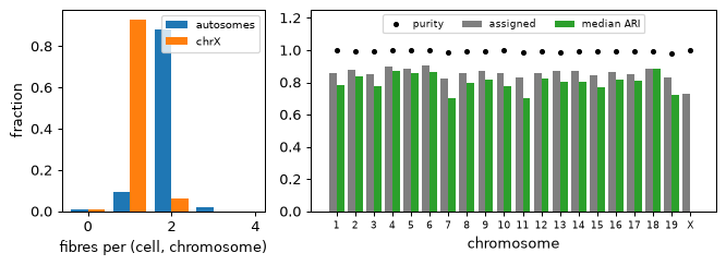
jie recovers the deposited assignment from geometry alone: almost every called fibre comes from one upstream homolog (purity ≈ 0.99), most labelled spots are placed, and the expected karyotype emerges — two copies of each autosome, one X. The losses are spots in long undetected stretches or ambiguous crowded regions; chrX has no ARI because the reference has a single label there.

5. Use the traced data

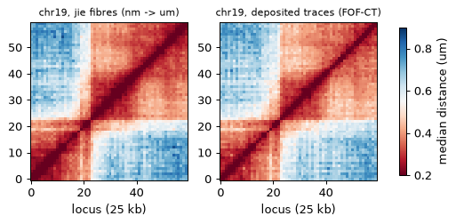
The result is an ordinary ChromData, so everything downstream applies. As a check, the population median distance map of chr19 from the jie fibres should match the one from the deposited traces of the same spots.

dm_jie = fea.distance_map(cd, "chr19")
ref = ChromData.from_fofct(FOFCT)
dm_ref = fea.distance_map(ref.get_chrom("chr19"), "chr19")
iu = np.triu_indices(dm_jie.matrix.shape[0], 1)
r = np.corrcoef(dm_jie.matrix[iu], dm_ref.matrix[iu])[0, 1]
print(f"chr19 median distance maps ({dm_jie.matrix.shape[0]} loci): Pearson r = {r:.3f} "
      f"(jie {dm_jie.n_traces} fibres, FOF-CT {dm_ref.n_traces} traces)")

fig, axes = plt.subplots(1, 2, figsize=(7, 3))
for ax, mat, title in [(axes[0], dm_jie.matrix / 1000, "jie fibres (nm -> um)"),
                       (axes[1], dm_ref.matrix, "deposited traces (FOF-CT)")]:
    im = ax.imshow(mat, cmap="RdBu", vmin=0.2, vmax=0.9, origin="lower", interpolation="nearest")
    ax.set_title(f"chr19, {title}", fontsize=9); ax.set_xlabel("locus (25 kb)")
fig.colorbar(im, ax=axes, shrink=0.8, label="median distance (um)")
plt.show()

chr19 median distance maps (60 loci): Pearson r = 0.990 (jie 373 fibres, FOF-CT 460 traces)

cd.uns["xyz_unit"] = "nm"
cd.uns["source"] = "Takei et al. 2021, Zenodo 3735329 (25-kb replicate 1), traced with uchrom.im.trace.align_spots"
cd.write(OUT / "takei2021_jie.chromdata.zarr")
print("wrote", OUT / "takei2021_jie.chromdata.zarr")

wrote _out/takei2021_jie.chromdata.zarr

Notes and next steps

• Parameters matter: calibrate max_skip / gap_penalty / min_spots_per_fiber to the detection efficiency of your data (section 3), ideally against a subset with a trusted assignment. τ is fitted per chromosome when not given.

• jie assumes the genome order is preserved in 3-D chains, so it is blind to structural variants (inversions, translocations); sisters closer than the localisation error (~150 nm) are merged into one fibre.

• Runtime grows with the candidates per locus; (cell, chromosome) graphs are independent, so large data can be split over processes.

• Next: import_fofct.ipynb (the traced table of this experiment), fish_imputation.ipynb (fill the loci a fibre missed), fishnet_domains.ipynb / tad_calling.ipynb (domains on traces).