Joint Hi-C + FISH reconstruction with GEM-FISH

Hi-C gives contacts along a whole chromosome; chromatin tracing gives real distances (in nm) for a small region. GEM-FISH (Abbas et al. 2019, Nat Commun 10:2049, doi:10.1038/s41467-019-10005-6) fuses the two into one 3-D model of a chromosome. This tutorial runs U-Chrom’s independent PyTorch re-implementation, uchrom.recon.fish.reconstruct_gem_fish, on real data from the same cell line, compares it with a Hi-C-only model to see what the imaging adds, and checks the result against the FISH distances and the Hi-C map.

Data: Rao et al. 2014, Cell 159:1665 (in situ Hi-C, IMR90, GEO GSE63525), chr21 at 5 kb, hg19 — ds.fetch("rao2014_imr90_chr21") builds it once (a 3.8 MB .cool, by HTTP range reads of the GEO .hic); Bintu et al. 2018, Science 362:eaau1783 (chromatin tracing of IMR90 chr21:20.0–21.95 Mb hg19, 65 segments of 30 kb, 1,277 imaged chromosomes) — ds.fetch("bintu_imr90") downloads it once (2 MB, GitHub). Modules: uchrom.recon.fish (reconstruct_gem_fish, GEMFISHParams), uchrom.io.read_bintu_tracing, uchrom.fea.distance_map. Runtime: about 1 min on a laptop CPU.

import time
from pathlib import Path

import cooler
import matplotlib.pyplot as plt
import numpy as np
import pandas as pd
from scipy.spatial.distance import cdist
from scipy.stats import pearsonr, spearmanr

import uchrom.datasets as ds
from uchrom.fea import distance_map
from uchrom.io import read_bintu_tracing
from uchrom.recon.fish import GEMFISHParams, reconstruct_gem_fish

plt.rcParams["figure.dpi"] = 90

OUT = Path("_out") / "gem_fish_reconstruction"; OUT.mkdir(parents=True, exist_ok=True)   # outputs: tutorials/_out/ (ignored by git)

HIC_5KB = ds.fetch("rao2014_imr90_chr21")   # Rao 2014 IMR90 chr21, 5 kb, raw counts, hg19 (built once from the GEO .hic)
BINTU = ds.fetch("bintu_imr90")             # Bintu 2018 IMR90 chr21 tracing (GitHub; downloaded once)

The imaging input

read_bintu_tracing reads Bintu’s CSV (one row per segment and imaged chromosome, nm) into a ChromData: one trace per imaged chromosome, one bin per 30 kb segment. We place segment 1 at its hg19 position (chr21:20,000,032; hg38 18,627,714 per the Bintu repository) so that it matches the hg19 Hi-C. uchrom.fea.distance_map gives the population median distance of every segment pair.

START_HG19 = 20_000_032
fish = read_bintu_tracing(str(BINTU), chrom="chr21", start_bp=START_HG19, resolution_bp=30_000)
fish.uns["genome_assembly"] = "hg19"
dm = distance_map(fish, "chr21", stat="median")
D_fish = dm.matrix
print(fish)
print(f"median distance map: {D_fish.shape[0]} segments, {dm.n_traces:,} traces; "
      f"median pair observed in {np.median(dm.count[np.triu_indices(len(D_fish), 1)]):.0f} traces")

ChromData: n_spots=77797, n_traces=1277, n_cells=1277, n_bins=65
  spots:   ['chrom', 'start', 'end', 'trace_id', 'cell_id', 'bin_id']
  uns:     ['xyz_unit', 'genome_assembly', 'source']
median distance map: 65 segments, 1,277 traces; median pair observed in 1128 traces

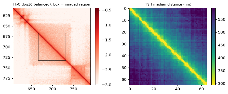
The Hi-C input on the same grid

To compare model and imaging bin by bin, the 5 kb Hi-C is summed into 30 kb bins whose edges fall on the Bintu segment grid (edges ≡ 20,000,000 mod 30 kb), so every FISH segment maps to exactly one Hi-C bin, and balanced with ICE.

def rebin_on_grid(src, out, chrom="chr21", res=30_000, anchor=START_HG19):
    # sum a fine cooler into `res` bins whose edges fall on the anchor's grid, then ICE-balance
    c = cooler.Cooler(str(src))
    L = int(c.chromsizes[chrom])
    phase = anchor // c.binsize * c.binsize % res
    edges = np.unique(np.r_[0, np.arange(phase, L, res), L])
    bins = pd.DataFrame({"chrom": chrom, "start": edges[:-1], "end": edges[1:]})
    px = c.pixels(join=True).fetch(chrom)
    b1 = np.searchsorted(edges, px["start1"].to_numpy(), side="right") - 1
    b2 = np.searchsorted(edges, px["start2"].to_numpy(), side="right") - 1
    agg = (pd.DataFrame({"bin1_id": b1, "bin2_id": b2, "count": px["count"].to_numpy()})
           .groupby(["bin1_id", "bin2_id"], as_index=False)["count"].sum())
    cooler.create_cooler(str(out), bins, agg, assembly="hg19", ordered=True)
    cooler.balance_cooler(cooler.Cooler(str(out)), store=True)
    return out


HIC = rebin_on_grid(HIC_5KB, OUT / "IMR90_chr21_30kb_bintu_grid.cool")
clr = cooler.Cooler(str(HIC))
H = np.nan_to_num(clr.matrix(balance=True).fetch("chr21"))
hic_bins = clr.bins().fetch("chr21")[["start", "end"]].to_numpy()
fish_mid = (dm.bins["start"].to_numpy() + dm.bins["end"].to_numpy()) // 2
fish_idx = np.searchsorted(hic_bins[:, 1], fish_mid, side="right")        # Hi-C bin of every FISH segment
assert len(set(fish_idx)) == len(fish_idx)
print(f"{HIC}: {clr.info['nbins']} bins x 30 kb, {clr.info['sum']:,} contacts; "
      f"FISH segments = Hi-C bins {fish_idx[0]}-{fish_idx[-1]}")

lo, hi = fish_idx[0] - 60, fish_idx[-1] + 60
fig, ax = plt.subplots(1, 2, figsize=(8.5, 3.5))
im = ax[0].imshow(np.log10(H[lo:hi, lo:hi] + 1e-4), cmap="Reds", vmin=-3,
                  extent=[lo - 0.5, hi - 0.5, hi - 0.5, lo - 0.5])
ax[0].add_patch(plt.Rectangle((fish_idx[0] - 0.5, fish_idx[0] - 0.5), len(fish_idx), len(fish_idx),
                              fill=False, ec="k", lw=1))
ax[0].set_title("Hi-C (log10 balanced); box = imaged region", fontsize=9); fig.colorbar(im, ax=ax[0], fraction=0.046)
VMIN, VMAX = np.nanpercentile(D_fish[np.triu_indices(len(D_fish), 1)], [1, 98])
im = ax[1].imshow(D_fish, cmap="viridis_r", vmin=VMIN, vmax=VMAX); ax[1].set_title("FISH median distance (nm)", fontsize=9)
fig.colorbar(im, ax=ax[1], fraction=0.046)
fig.tight_layout()

_out/gem_fish_reconstruction/IMR90_chr21_30kb_bintu_grid.cool: 1605 bins x 30 kb, 10,266,877 contacts; FISH segments = Hi-C bins 667-731

Running GEM-FISH

reconstruct_gem_fish works in three stages (per chromosome):

1. TAD level — partition the chromosome into TADs (Dixon directionality-index caller, or tads=) and place the TAD centres by gradient descent on Hi-C KL divergence + polymer prior (λ_E) + FISH inter-TAD distances (λ_F, in nm).

2. Inside every TAD — place its bins on intra-TAD Hi-C + polymer prior + the FISH radius of gyration of the TAD (λ_R).

3. Assembly — move every TAD to its centre and rotate it to join its neighbours.

FISH can only act through TAD-centre distances and TAD sizes, so the imaged region must span several TADs. With the default cap (TADs of at most 5 % of the chromosome, 80 bins = 2.4 Mb) the DI caller’s TADs are as large as the whole imaged region, which then falls into one or two TADs and the FISH terms barely change the model. We cap them at 1 % (16 bins, 480 kb; tad_max_size_frac=0.01): the imaged region then holds five TADs. The λ weights are this tutorial’s settings, not tuned here; the optimiser is seeded, so a CPU run is reproducible.

params = GEMFISHParams(lambda_E_tad=0.5, lambda_F=0.5, lambda_E_intra=0.05, lambda_R=0.01,
                       stage1_iter=500, stage1_ensemble=20, stage2_iter=300, stage2_ensemble=6,
                       tad_di_window=50, tad_di_min_size_frac=0.01, tad_max_size_frac=0.01,
                       device="cpu", verbose=False)
t0 = time.time()
gf, parts = reconstruct_gem_fish(hic_path=str(HIC), chrom="chr21", fish_cd=fish, params=params,
                                 return_intermediate=True)
t_gf = time.time() - t0
tads = parts["tad_windows"]
in_region = [(s, e) for s, e in tads if e > fish_idx[0] and s <= fish_idx[-1]]
print(f"GEM-FISH: {t_gf:.0f} s, {len(tads)} TADs, {len(in_region)} of them in the imaged region: {in_region}")
print(gf)
print(gf.uns["gem_fish"])

GEM-FISH: 23 s, 106 TADs, 5 of them in the imaged region: [(664, 680), (680, 693), (693, 709), (709, 725), (725, 741)]
ChromData: n_spots=1605, n_traces=1, n_bins=1605
  spots:   ['chrom', 'start', 'end', 'trace_id', 'bin_id']
  uns:     ['gem_fish', 'xyz_unit', 'genome_assembly']
{'n_tads': 106, 'stage1_final_loss': 777045.4835715899, 'stage1_best_ensemble': 3}

The result is a ChromData with one spot per Hi-C bin and one trace (a single consensus model); return_intermediate=True also returns the stage outputs (TAD windows and centres, per-TAD coordinates, the FISH targets, loss histories).

For comparison, the same run without imaging (fish_cd=None, a Hi-C-only model):

t0 = time.time()
hic_only = reconstruct_gem_fish(hic_path=str(HIC), chrom="chr21", fish_cd=None, params=params)
print(f"Hi-C only: {time.time() - t0:.0f} s; final stage-1 loss {hic_only.uns['gem_fish']['stage1_final_loss']:.3g} "
      f"(with FISH: {gf.uns['gem_fish']['stage1_final_loss']:.3g})")
gf.write(OUT / "IMR90_chr21_gemfish.chromdata.zarr")
hic_only.write(OUT / "IMR90_chr21_hic_only.chromdata.zarr")

Hi-C only: 23 s; final stage-1 loss 96 (with FISH: 7.77e+05)

Agreement with the imaged distances

Map every FISH segment to its model bin, compare the model distance matrix with the FISH median distances (Pearson r) and compute GEM-FISH’s error measure, the mean relative error |s·d_model − d_FISH| / d_FISH after rescaling the model by the least-squares factor s (scale_nm, nm per model unit). For the GEM-FISH model the same FISH data were restraints, so this is a fit, not a held-out score; the Hi-C-only model never saw them.

def fish_scores(cd):
    loci = cd.spots_with_loci()
    starts, ends = loci["start"].to_numpy(), loci["end"].to_numpy()
    idx = np.array([np.flatnonzero((starts <= m) & (ends > m))[0] for m in fish_mid])
    D = cdist(cd.coords[idx], cd.coords[idx])
    iu = np.triu_indices(len(idx), 1)
    f, m = D_fish[iu], D[iu]
    ok = np.isfinite(f)
    f, m = f[ok], m[ok]
    s = (m / f).sum() / ((m / f) ** 2).sum()
    return {"pearson": pearsonr(f, m)[0], "rel_error": float(np.mean(np.abs(s * m - f) / f)), "scale_nm": s}, D * s


pd.DataFrame({name: fish_scores(cd)[0] for name, cd in (("Hi-C + FISH", gf), ("Hi-C only", hic_only))}).T.round(3)

	pearson	rel_error	scale_nm
Hi-C + FISH	0.750	0.327	20.758
Hi-C only	0.675	0.277	48.148

Agreement with the Hi-C map

The model should also reproduce the contact map: high contact frequency ↔ short distance. Over the whole chromosome we compute the Spearman correlation between the balanced contacts and 1 / d, raw and after removing the distance decay (observed / expected on both sides), for all pairs and for pairs within 3 Mb.

def observed_over_expected(A):
    n = len(A); out = np.full_like(A, np.nan, dtype=float)
    for k in range(1, n):
        i = np.arange(n - k); v = A[i, i + k]; pos = v > 0
        if pos.any():
            out[i, i + k] = out[i + k, i] = np.where(pos, v / v[pos].mean(), np.nan)
    return out


def hic_scores(cd):
    loci = cd.spots_with_loci()
    rows = np.searchsorted(hic_bins[:, 0], loci["start"].to_numpy())          # model bin -> Hi-C bin
    Hm = H[np.ix_(rows, rows)]
    D = cdist(cd.coords, cd.coords)
    iu = np.triu_indices(len(rows), 1)
    near = (np.abs(rows[iu[0]] - rows[iu[1]]) * 30_000) <= 3_000_000
    Hoe, Doe = observed_over_expected(Hm), observed_over_expected(D)
    out = {}
    for label, sel in (("all pairs", np.ones_like(near)), ("<= 3 Mb", near)):
        ok = sel & (Hm[iu] > 0)
        out[f"raw, {label}"] = spearmanr(Hm[iu][ok], 1 / D[iu][ok])[0]
        ok = sel & np.isfinite(Hoe[iu]) & (Hoe[iu] > 0) & np.isfinite(Doe[iu])
        out[f"O/E, {label}"] = spearmanr(Hoe[iu][ok], 1 / Doe[iu][ok])[0]
    return out


pd.DataFrame({name: hic_scores(cd) for name, cd in (("Hi-C + FISH", gf), ("Hi-C only", hic_only))}).T.round(3)

	raw, all pairs	O/E, all pairs	raw, <= 3 Mb	O/E, <= 3 Mb
Hi-C + FISH	-0.029	-0.085	0.057	-0.124
Hi-C only	0.407	0.168	0.702	0.311

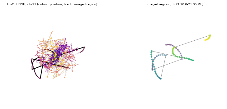
The Hi-C-only model follows the contact map; the FISH-constrained one loses it over the whole chromosome. The FISH term of stage 1 compares model distances, in units of order 1, with FISH distances in nm: it dominates the stage-1 loss (printed above: about 8 × 10⁵ with FISH, about 10² without), so the arrangement of all 106 TAD centres is driven by the five imaged ones instead of by the Hi-C. In 3-D the imaged region (black) is stretched out at the edge of an otherwise compact chromosome:

from mpl_toolkits.mplot3d import Axes3D  # noqa: F401 (registers the 3-D projection)

loci = gf.spots_with_loci()
region = ((loci["end"] > START_HG19) & (loci["start"] < dm.bins["end"].max())).to_numpy()
fig = plt.figure(figsize=(9, 4))
ax = fig.add_subplot(1, 2, 1, projection="3d")
X = gf.coords
ax.plot(*X.T, lw=0.4, color="0.7")
ax.scatter(*X.T, c=np.arange(len(X)), cmap="plasma", s=1.5)
ax.plot(*X[region].T, lw=2, color="k")
ax.set_title("Hi-C + FISH, chr21 (colour: position; black: imaged region)", fontsize=8); ax.set_axis_off()
ax = fig.add_subplot(1, 2, 2, projection="3d")
Z = X[region]
ax.plot(*Z.T, lw=0.8, color="0.5"); ax.scatter(*Z.T, c=np.arange(len(Z)), cmap="viridis", s=12)
ax.set_title("imaged region (chr21:20.0-21.95 Mb)", fontsize=8); ax.set_axis_off()
fig.tight_layout()

Modelling only the imaged TADs

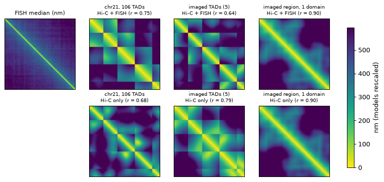
In the GEM-FISH paper every modelled TAD was imaged (Wang et al. 2016 traced TAD centres along whole chromosomes). tads= (a table of start / end in bp) sets the partition and restricts the model to those windows, so we can reproduce that situation here: the five DI TADs that overlap the imaged region (from the run above), or the whole region as one domain. Every modelled TAD then has FISH data, as in the paper. Each run takes a few seconds.

runs = {(f"chr21, {len(tads)} TADs", "Hi-C + FISH"): gf, (f"chr21, {len(tads)} TADs", "Hi-C only"): hic_only}
t0 = time.time()
for label, windows in (("imaged TADs (5)", in_region), ("imaged region, 1 domain", [(in_region[0][0], in_region[-1][1])])):
    tads_bp = pd.DataFrame({"start": [hic_bins[s, 0] for s, e in windows], "end": [hic_bins[e - 1, 1] for s, e in windows]})
    for inputs, f in (("Hi-C + FISH", fish), ("Hi-C only", None)):
        runs[(label, inputs)] = reconstruct_gem_fish(hic_path=str(HIC), chrom="chr21", fish_cd=f, tads=tads_bp, params=params)
print(f"4 region models in {time.time() - t0:.0f} s, {runs[('imaged TADs (5)', 'Hi-C only')].n_spots} bins each "
      f"(chr21:{hic_bins[in_region[0][0], 0]:,}-{hic_bins[in_region[-1][1] - 1, 1]:,})")

rows, mats = [], {}
for (model, inputs), cd in runs.items():
    fs, mats[(model, inputs)] = fish_scores(cd)
    hs = hic_scores(cd)
    rows.append({"model": model, "inputs": inputs, "r vs FISH": fs["pearson"], "rel. error vs FISH": fs["rel_error"],
                 "Spearman vs Hi-C": hs["raw, all pairs"], "Spearman vs Hi-C (O/E)": hs["O/E, all pairs"]})
summary = pd.DataFrame(rows).set_index(["model", "inputs"])
summary.round(3)

4 region models in 6 s, 77 bins each (chr21:19,910,000-22,220,000)

		r vs FISH	rel. error vs FISH	Spearman vs Hi-C	Spearman vs Hi-C (O/E)
model	inputs
chr21, 106 TADs	Hi-C + FISH	0.750	0.327	-0.029	-0.085
	Hi-C only	0.675	0.277	0.407	0.168
imaged TADs (5)	Hi-C + FISH	0.643	0.290	0.608	0.025
	Hi-C only	0.793	0.414	0.823	0.066
imaged region, 1 domain	Hi-C + FISH	0.900	0.298	0.850	0.056
	Hi-C only	0.901	0.297	0.851	0.057

models = list(dict.fromkeys(m for m, _ in runs))
fig, axes = plt.subplots(2, len(models) + 1, figsize=(10, 4.6))
axes[0, 0].imshow(D_fish, cmap="viridis_r", vmin=0, vmax=VMAX); axes[0, 0].set_title("FISH median (nm)", fontsize=9)
axes[1, 0].set_axis_off()
for c, model in enumerate(models, start=1):
    for r, inputs in enumerate(("Hi-C + FISH", "Hi-C only")):
        im = axes[r, c].imshow(mats[(model, inputs)], cmap="viridis_r", vmin=0, vmax=VMAX)
        axes[r, c].set_title(f"{model}\n{inputs} (r = {summary.loc[(model, inputs), 'r vs FISH']:.2f})", fontsize=8)
for ax in axes.flat:
    ax.set_xticks([]); ax.set_yticks([])
cb = fig.colorbar(im, ax=axes, fraction=0.02, label="nm (models rescaled)")

Notes and caveats

• What the imaging adds — on this data, little. Over the imaged region the Hi-C-only models match the imaged distances as well as or better than the FISH-constrained ones (summary table: r 0.79 vs 0.64 with the five imaged TADs, 0.90 vs 0.90 with the region as one domain). FISH lowers the relative error of the five-TAD model (0.41 → 0.29) and raises r of the whole-chromosome model (0.68 → 0.75), at the cost described next. With the default TAD cap (5 %) the region falls into one or two TADs and FISH changes r by less than 0.01 (0.705 → 0.710 in a run not shown). The FISH data are restraints here, so no FISH score is held out — and still the Hi-C alone does as well; the closest description of the imaged distances is the Hi-C model of the region as one domain.

• Partial FISH coverage distorts the whole model. With FISH for a few TADs of a whole chromosome, the nm-valued FISH term dominates the TAD-level loss and the assembled model no longer reproduces the Hi-C. This re-implementation does not balance the FISH term against the unit-scale terms (λ_F is an absolute weight); model only imaged TADs (tads=), or use the Hi-C-only model outside the imaged region.

• Assembly is a one-anchor Kabsch rotation per TAD, a simplification of the paper’s gradient-descent assembly; it leaves visible jumps between consecutive TADs (the block pattern of the distance maps).

• Weights. The paper’s λ values (λ_E = 5 × 10¹², λ_F = 10⁻⁸) are for raw counts without row normalisation; this re-implementation row-normalises inside the KL term, so its weights differ.

• Not a benchmark. The paper’s evaluation (Wang 2016 TAD-centre FISH, TAD-level distances) is benchmarks/fig3/c_gemfish_wang2016.py.

• Other chromosomes are sliced from the same Rao 2014 map the same way as chr21 here (uchrom.datasets._builders.slice_hic(cell="IMR90", chroms=["20"], res=5000, out=...), HTTP range reads of the GEO .hic). Do not pair IMR90 imaging with K562 Hi-C (rao2014_k562_chr21).

• Device: device="auto" uses CUDA / Apple MPS; results then differ from the CPU run (float32 and a different random stream).

Supplement (synthetic data): the three stages on a known structure

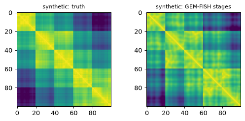
This part uses a simulated chain, not real data. It shows the mechanics of the three stages with a ground truth to compare against — five compact TADs, contacts generated as 1 / (1 + d), noisy FISH centre distances and radii of gyration — through the internal stage functions that reconstruct_gem_fish chains together.

from uchrom.recon.fish._assembly import assemble
from uchrom.recon.fish._hic import contact_to_distance
from uchrom.recon.fish._intra_tad import Stage2Params, reconstruct_intra_tad
from uchrom.recon.fish._tad_level import Stage1Params, reconstruct_tad_level

rng = np.random.default_rng(0)
n_tads, per_tad = 5, 20
truth, centre = [], np.zeros(3)
for t in range(n_tads):
    walk = np.cumsum(rng.normal(0, 0.3, (per_tad, 3)), axis=0)
    truth.append(walk - walk.mean(0) + centre)
    centre = centre + 5.0 * (np.array([1.0, 0, 0]) + 0.3 * rng.normal(0, 1, 3))
truth = np.vstack(truth)
windows = [(t * per_tad, (t + 1) * per_tad) for t in range(n_tads)]
D_true = cdist(truth, truth)
contacts_syn = 1.0 / (1.0 + D_true); np.fill_diagonal(contacts_syn, 0)
inter = np.array([[contacts_syn[a:b, c:d].sum() for c, d in windows] for a, b in windows])
centres_true = np.array([truth[a:b].mean(0) for a, b in windows])
F = cdist(centres_true, centres_true) + rng.normal(0, 0.1, (n_tads, n_tads)); np.fill_diagonal(F, 0)
rg2 = [((truth[a:b] - truth[a:b].mean(0)) ** 2).sum(1).mean() * (1 + 0.05 * rng.standard_normal()) for a, b in windows]

centres, _ = reconstruct_tad_level(inter, F, params=Stage1Params(lambda_E=0.05, lambda_F=0.5, n_iter=500,
                                                                   n_ensemble=20, device="cpu"))
intra, _ = reconstruct_intra_tad(contacts_syn, windows, target_rg_sq_per_tad=rg2,
                                 params=Stage2Params(lambda_E=0.05, lambda_R=0.01, n_iter=300, n_ensemble=6, device="cpu"))
mid = np.array([(a + b - 1) / 2 * per_tad for a, b in windows])
gap = contact_to_distance(inter, genomic_distances=np.abs(mid[:, None] - mid[None]).astype(float),
                          alpha=0.25, fallback_c=1.0, fallback_beta=0.5)
final = assemble(centres, intra, inter_tad_distances=gap)

iu5, iuN = np.triu_indices(n_tads, 1), np.triu_indices(len(truth), 1)
print(f"stage 1, TAD-centre distances vs truth: r = {np.corrcoef(cdist(centres, centres)[iu5], cdist(centres_true, centres_true)[iu5])[0, 1]:.3f}")
print(f"stage 2, mean intra-TAD distance r = "
      f"{np.mean([np.corrcoef(cdist(intra[k], intra[k])[np.triu_indices(per_tad, 1)], D_true[a:b, a:b][np.triu_indices(per_tad, 1)])[0, 1] for k, (a, b) in enumerate(windows)]):.3f}")
print(f"assembled chain, all distances vs truth: r = {np.corrcoef(cdist(final, final)[iuN], D_true[iuN])[0, 1]:.3f}")
fig, ax = plt.subplots(1, 2, figsize=(6, 2.8))
for a, (title, M) in zip(ax, [("truth", D_true), ("GEM-FISH stages", cdist(final, final))]):
    a.imshow(M, cmap="viridis_r", vmax=np.percentile(D_true, 98)); a.set_title(f"synthetic: {title}", fontsize=9)
fig.tight_layout()

stage 1, TAD-centre distances vs truth: r = 1.000
stage 2, mean intra-TAD distance r = 0.925
assembled chain, all distances vs truth: r = 0.910

Next steps

• bulk_reconstruction — the same Hi-C map with MDS and IGM population deconvolution, checked against the same tracing data.

• reconstruction — single-cell Hi-C to 3-D (NucDynamics, EMber).

• tad_calling, fish_imputation — more analyses of chromatin-tracing data.