Loop calling on chromatin tracing data

This tutorial calls chromatin loops from DNA FISH traces with uchrom.strc.loop.call_loops_axiswise_f (also uc.tl.call_loops), an independent GPU-capable implementation of the axis-wise F-test of ArcFISH (Yu et al. 2025, bioRxiv 10.1101/2025.11.26.690837). You will call loops on one chromosome and on all of them at once, check the calls against the population distance and contact maps (uchrom.fea, uchrom.pl), tune LoopCallerParams, and keep the calls in cd.intervals / cd.results and on disk. Data: Takei et al. 2021 (Nature 590:344) DNA seqFISH+ in mouse ES cells at 25 kb — 20 regions of 60 loci (1.5–2.4 Mb), one per chromosome, 8,285 traces in 201 cells (ds.fetch("takei") downloads the FOF-CT core table 4DNFIHF3JCBY once from 4DN, 22 MB). Runtime: about a minute.

How the caller works (per chromosome):

1. Per-axis variance — for each bin pair (i, j) and each axis, the variance of x[j] - x[i] across traces. Modelling the axes separately absorbs the anisotropic localisation error of FISH (z is usually noisier).

2. Filter + normalise — LOWESS on log genomic distance removes per-trace outliers (4 σ) and divides out the distance decay.

3. Per-axis F-test — a candidate pair is compared with a local background ring 25–50 kb away; a loop has lower variance than its ring.

4. ACAT — the three per-axis p-values are combined with weights ∝ 1 / (median per-trace variance of that axis).

5. BH-FDR, clustering of accepted pairs within 50 kb, and the lowest-p summit of each cluster.

6. Contact filter — a summit is kept when more than 1/2 (singletons) or 1/3 (clusters) of the traces bring its anchors closer than the typical distance of adjacent loci.

import shutil
import time
from pathlib import Path

import numpy as np
import pandas as pd
import matplotlib.pyplot as plt

from chromdata import ChromData
import uchrom as uc
import uchrom.datasets as ds

plt.rcParams["figure.dpi"] = 90

OUT = Path("_out"); OUT.mkdir(exist_ok=True)   # outputs: tutorials/_out/ (ignored by git)
CORE = ds.fetch("takei")                       # Takei 2021 FOF-CT core table (4DN, 22 MB; downloaded once)

Load the Takei 2021 traces

ChromData.from_fofct reads the 4DN FISH Omics Format (FOF-CT) core table; the loci become cd.bins, every detected spot a row of cd.spots.

cd = ChromData.from_fofct(CORE)
print(cd)
per_chrom = pd.DataFrame({
    "loci": cd.bins.groupby("chrom", observed=True).size(),
    "traces": cd.spots.groupby("chrom", observed=True)["trace_id"].nunique(),
})
per_chrom.T

ChromData: n_spots=316995, n_traces=8285, n_cells=201, n_bins=1200
  spots:   ['chrom', 'start', 'end', 'trace_id', 'spot_id', 'cell_id', 'extra_cell_roi_id', 'bin_id']
  uns:     ['fofct_header', 'xyz_unit', 'genome_assembly']

chrom	chr1	chr10	chr11	chr12	chr13	chr14	chr15	chr16	chr17	chr18	chr19	chr2	chr3	chr4	chr5	chr6	chr7	chr8	chr9	chrX
loci	60	60	60	60	60	60	60	60	60	60	60	60	60	60	60	60	60	60	60	60
traces	424	418	442	424	430	416	400	421	427	445	460	418	408	423	406	415	430	438	423	217

Call loops on one chromosome

chrom="chr6" restricts the call to one chromosome. The defaults follow ArcFISH (fdr_cutoff=0.1, pval_cutoff=1e-5, candidates 100 kb–1 Mb apart, background ring 25–50 kb, clustering gap 50 kb); device="auto" picks CUDA, then Apple MPS, then the CPU.

from uchrom.strc.loop import call_loops_axiswise_f, LoopCallerParams

COLS = ["chrom1", "start1", "end1", "start2", "end2", "pval", "fdr", "cluster_size", "contact_freq"]
loops6 = call_loops_axiswise_f(cd, chrom="chr6", verbose=True)
loops6[COLS]

[loop/chr6] computing axis variance cube...

[loop/chr6] 415 traces, 60 bins; normalising...
[loop/chr6] axis weights x=0.335, y=0.330, z=0.335
[loop/chr6] median bin size 25000 bp, ring bins [1, 2]
[loop/chr6] 1397 candidates; running F-test...

	chrom1	start1	end1	start2	end2	pval	fdr	cluster_size	contact_freq
0	chr6	50300000	50325000	50525000	50550000	0.000004	0.002537	4	0.557471

The table is BEDPE-like (one row per loop summit). It is stored, with its provenance, under the default key "loops.axiswise_f": as a typed pair interval table in cd.intervals and as a record in cd.results.

print(cd.intervals)
rec = cd.results.record("loops.axiswise_f")
print(rec.function, "| kind:", rec.kind)
print("params:", rec.params)

IntervalStore({'loops.axiswise_f': <pair, 1 rows>})
uchrom.strc.loop.call_loops_axiswise_f | kind: intervals
params: {'cut_lo': 100000.0, 'cut_up': 1000000.0, 'inner_cut': 25000.0, 'outer_cut': 50000.0, 'fdr_cutoff': 0.1, 'pval_cutoff': 1e-05, 'gap': 50000.0, 'k_sigma': 4.0, 'frac': 0.1, 'min_cluster_size': 1}

ArcFISH’s own tutorial runs LoopCaller(fdr_cutoff=0.1) on this chromosome of the same dataset and reports two loops. Which of them does this implementation find (anchors within one 25-kb bin)?

# ArcFISH documentation, tutorial "Loop and domain calling" (Takei 2021 25-kb data, chr6)
arcfish_chr6 = pd.DataFrame({"start1": [50_300_000, 50_675_000], "start2": [50_525_000, 50_800_000]})


def found(ref, calls, tol=25_000):
    return [bool(((calls.start1 - a).abs().le(tol) & (calls.start2 - b).abs().le(tol)).any())
            for a, b in zip(ref.start1, ref.start2)]


arcfish_chr6.assign(called_here=found(arcfish_chr6, loops6))

	start1	start2	called_here
0	50300000	50525000	True
1	50675000	50800000	False

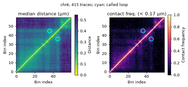
Check the call against the population maps

A loop is a pair of loci that are closer than their genomic separation predicts, i.e. a dot off the diagonal of the median distance map and of the contact-frequency map. uchrom.fea.distance_map gives the exact median over traces (in memory or streaming over a backed store); contact_frequency counts the traces in which a pair is closer than a cutoff — here the median distance of adjacent loci, the same kind of cutoff the caller’s contact filter uses.

from uchrom.fea import contact_frequency, distance_map
from uchrom.pl import plot_contact_map, plot_distance_matrix

dm = distance_map(cd, "chr6")                               # median over traces, µm
row = {s: k for k, s in enumerate(dm.bins["start"])}        # locus start -> matrix row
cutoff = float(np.nanmedian(np.diag(dm.matrix, 1)))
cf, _, _ = contact_frequency(cd.get_chrom("chr6").to_dataframe(), threshold=cutoff, chrom="chr6")

fig, axes = plt.subplots(1, 2, figsize=(7, 3.1))
plot_distance_matrix(dm.matrix, title=f"median distance (µm)", ax=axes[0])
plot_contact_map(cf, title=f"contact freq. (< {cutoff:.2f} µm)", ax=axes[1])
fig.suptitle(f"chr6, {dm.n_traces} traces; cyan: called loop", fontsize=10)
for ax in axes:
    for _, r in loops6.iterrows():
        i, j = row[r.start1], row[r.start2]
        ax.plot([j, i], [i, j], "o", mfc="none", mec="cyan", mew=1.5, ms=11)
plt.tight_layout(); plt.show()

All chromosomes at once

With chrom=None (the default) the caller runs every chromosome and merges the per-chromosome tables into one table under one key — here through the flat alias uc.tl.call_loops, which forwards to the same function.

t0 = time.perf_counter()
loops = uc.tl.call_loops(cd)
print(f"{len(loops)} loops on {loops.chrom1.nunique()} of {cd.bins.chrom.nunique()} chromosomes "
      f"({time.perf_counter() - t0:.1f} s)")
loops[COLS]

5 loops on 5 of 20 chromosomes (5.0 s)

	chrom1	start1	end1	start2	end2	pval	fdr	cluster_size	contact_freq
0	chr12	63200000	63225000	63300000	63325000	1.128507e-07	1.210888e-04	1	0.626556
1	chr2	109900000	109925000	110200000	110225000	7.145620e-10	9.846665e-07	4	0.543860
2	chr4	90550000	90575000	90700000	90725000	9.020898e-08	1.159185e-04	1	0.575130
3	chr6	50300000	50325000	50525000	50550000	3.632526e-06	2.537320e-03	4	0.557471
4	chrX	75375457	75400457	75775457	75800457	9.646543e-06	1.272379e-02	1	0.555556

fig, axes = plt.subplots(2, 3, figsize=(7, 4.9))
for ax, (_, r) in zip(axes.flat, loops.iterrows()):
    d = distance_map(cd, r.chrom1)
    k = {s: q for q, s in enumerate(d.bins["start"])}
    ax.imshow(d.matrix, cmap="viridis_r", origin="lower")
    ax.plot([k[r.start2]], [k[r.start1]], "o", mfc="none", mec="cyan", mew=1.5, ms=10)
    ax.set_title(f"{r.chrom1} {r.start1 / 1e6:.3f} ↔ {r.start2 / 1e6:.3f} Mb", fontsize=8)
    ax.set_xticks([]); ax.set_yticks([])
for ax in axes.flat[len(loops):]:
    ax.axis("off")
fig.suptitle("Called loops on the median distance maps", fontsize=10)
plt.tight_layout()
plt.show()

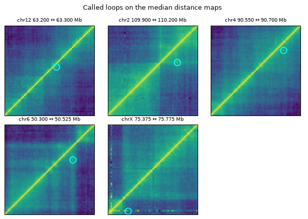
How this compares with the paper. On this dataset the ArcFISH preprint reports 25 loops, 17 of them supported by Hi-C / PLAC-seq / ChIA-PET loop lists (SnapFISH: 41 loops, 23 supported). With the same default thresholds this implementation is more conservative: the five summits above. The next section shows how the call set grows when the thresholds are relaxed.

Tuning the thresholds

Every knob lives on LoopCallerParams. key_added=None returns the table without storing it, so the default call above stays in cd.intervals.

settings = {
    "default (fdr 0.1, p 1e-5)": LoopCallerParams(),
    "p 1e-3": LoopCallerParams(pval_cutoff=1e-3),
    "fdr 0.2, p 1e-3": LoopCallerParams(fdr_cutoff=0.2, pval_cutoff=1e-3),
}
counts = {name: (loops if name.startswith("default") else
                 uc.tl.call_loops(cd, params=p, key_added=None)).groupby("chrom1").size()
          for name, p in settings.items()}
table = pd.DataFrame(counts).fillna(0).astype(int)
table.loc["total"] = table.sum()
table.T

chrom1	chr12	chr13	chr16	chr19	chr2	chr3	chr4	chr6	chrX	total
default (fdr 0.1, p 1e-5)	1	0	0	0	1	0	1	1	1	5
p 1e-3	1	2	2	1	1	4	1	2	1	15
fdr 0.2, p 1e-3	1	2	4	2	1	4	1	2	3	20

relaxed6 = uc.tl.call_loops(cd, chrom="chr6", params=settings["p 1e-3"], key_added=None)
arcfish_chr6.assign(called_at_p_1e_3=found(arcfish_chr6, relaxed6))

	start1	start2	called_at_p_1e_3
0	50300000	50525000	True
1	50675000	50800000	True

copy=True: leave the input untouched

By default the caller writes into cd and returns the table. With copy=True it returns a new ChromData that holds the result instead.

cd_chr2 = uc.tl.call_loops(cd, chrom="chr2", key_added="loops.chr2", copy=True)
print(type(cd_chr2).__name__, "intervals:", list(cd_chr2.intervals))
print("'loops.chr2' in the original:", "loops.chr2" in cd.intervals)

ChromData intervals: ['loops.axiswise_f', 'loops.chr2']
'loops.chr2' in the original: False

Save and reload

Interval tables and result records travel with the .chromdata.zarr store; a backed read loads them eagerly while the coordinates stay on disk. For other tools, export BEDPE.

path = OUT / "takei2021_loops.chromdata.zarr"
if path.exists():
    shutil.rmtree(path)
cd.write(path)

back = ChromData.read(path, backed=True)
print(back.intervals)
print(back.results.record("loops.axiswise_f").created_utc)

bedpe = OUT / "takei2021_loops.bedpe"
back.intervals["loops.axiswise_f"][["chrom1", "start1", "end1", "chrom2", "start2", "end2", "score"]] \
    .to_csv(bedpe, sep="\t", header=False, index=False)
print("wrote", bedpe)

IntervalStore({'loops.axiswise_f': <pair, 5 rows>})
2026-10-06T22:52:19+00:00
wrote _out/takei2021_loops.bedpe

Command line

The same caller runs from the shell on a store or a FOF-CT table, writing BEDPE, CSV or an updated store:

python -m uchrom.strc.loop --input=data.chromdata.zarr --output=chr6_loops.bedpe --chrom=chr6

Notes

• The implementation is independent of the GPL-3.0 ArcFISH source; the per-trace 4 σ filter, LOWESS normalisation, per-axis F-test, ACAT, BH-FDR and the summit / contact-frequency rules are re-implemented.

• On Apple MPS the variance cube is computed in float32 (CUDA / CPU use float64), which can move borderline candidates across the thresholds.

• On a backed store the caller streams over the traces (streaming=True, memory O(n_bins²)); the tad_calling tutorial shows it.

Next steps

• tad_calling — ArcFISH TADs, streaming on a backed store, and projecting TADs / loops onto bins and spots with uchrom.strc.enrichment.

• fishnet_domains — single-allele domains with FISHnet.

• compartment — A/B compartments, validated against Hi-C.