Importing seqFISH+ multi-omics data (Takei 2025 cerebellum)

DNA seqFISH+ multi-omics images ~100,000 genomic loci per nucleus at 25 kb resolution together with dozens of immunofluorescence (IF) and RNA channels, so every DNA spot carries its own chromatin-mark signals. In this tutorial you import such data with uchrom.io.read_seqfish_multiomics and walk through how it maps onto ChromData: the locus panel (bins), spots and traces, the 62 per-spot signals (spot_tracks), cells with types, positions and a UMAP (cells, cellm), per-trace quality (traces) and metadata (uns). You also stream the import into a store (out=) and open the full replicate backed from the public U-Chrom atlas.

Data: Takei et al. 2025, Nature (doi:10.1038/s41586-025-08838-x), adult mouse cerebellum, Zenodo 7693825; locus map and cell clustering from the authors’ repository CaiGroup/dna-seqfish-plus-multi-omics. We import the first 47 cells of replicate 1, field of view 0: ds.fetch("takei2025_fov0") streams the start of that FOV’s CSV (47 whole cells, 0.27 GB) out of the Zenodo tarball and downloads the two tables from GitHub, once. The last section opens the whole replicate (1,799 cells, 10.9 M spots) from the atlas over HTTP. Runtime: about a minute.

from pathlib import Path
import time

import numpy as np
import pandas as pd
import matplotlib.pyplot as plt
from scipy.stats import spearmanr
from chromdata import ChromData
import uchrom.datasets as ds
from uchrom.io import read_seqfish_multiomics
from uchrom.io.seqfish_multiomics import IF_COLUMNS
from uchrom.emb import aggregate_tracks

plt.rcParams["figure.dpi"] = 90

OUT = Path("_out"); OUT.mkdir(exist_ok=True)   # outputs: tutorials/_out/ (ignored by git)
FOV0 = ds.fetch("takei2025_fov0")              # folder; built once from Zenodo 7693825 + the authors' GitHub
SPOTS = FOV0 / "cerebellum_rep1_pos0_cells.csv"                  # 47 whole cells of rep 1 / FOV 0
LOCI = FOV0 / "LC1-100k-09022022-mm10-25kb-meta.csv"             # 25-kb locus map (GitHub)
CLUSTERS = FOV0 / "cerebellum_mRNA_cluster_nuc_vol_filtered.csv" # per-cell clustering (GitHub)
for p in (SPOTS, LOCI, CLUSTERS):
    print(f"{p.relative_to(ds.data_dir())}  ({p.stat().st_size / 1e6:.1f} MB)")

takei2025_fov0/cerebellum_rep1_pos0_cells.csv  (272.7 MB)
takei2025_fov0/LC1-100k-09022022-mm10-25kb-meta.csv  (7.5 MB)
takei2025_fov0/cerebellum_mRNA_cluster_nuc_vol_filtered.csv  (0.3 MB)

1. The input files

• Spot table (one CSV per field of view): one row per DNA spot with rep, fov, cellID, the locus name (e.g. chr7-1628), its position (x_um, y_um, z_um; x, y, z are voxels), three homolog (allele) assignments of increasing recall (dbscan_allele, dbscan_ldp_allele, dbscan_ldp_nbr_allele; −1 = unassigned) and 59 z-scored signals measured at the spot.

• Locus map: name → chrom, start, end (+ GC content, genes) for the whole probe panel.

• Cell clustering: per cell leiden cluster, the published RNA UMAP, nuclear centroid (voxels) and volume, doublet flag.

head = pd.read_csv(SPOTS, nrows=5)
print(f"{len(head.columns)} columns:", ", ".join(head.columns[:9]), "...", ", ".join(head.columns[-8:]))
head[["rep", "fov", "cellID", "name", "chrom", "x_um", "y_um", "z_um",
      "dbscan_ldp_nbr_allele", "H3K27ac", "LaminB1", "dot_int"]]

76 columns: rep, fov, cellID, x, y, z, dot_int, name, chrom ... dbscan_allele, dbscan_ldp_allele, dbscan_ldp_nbr_allele, x_um, y_um, z_um, n_rad_score, n_per_dist(um)

	rep	fov	cellID	name	chrom	x_um	y_um	z_um	dbscan_ldp_nbr_allele	H3K27ac	LaminB1	dot_int
0	1	0	270	chr7-1628	chr7	135.735563	105.863812	1.61650	-1	-1.20850	-0.84303	832
1	1	0	270	chr1-5057	chr1	135.981733	112.468790	1.60700	-1	-1.10850	-1.19330	339
2	1	0	270	chr10-1393	chr10	131.758424	107.129991	1.60600	1	-1.06140	-0.72628	469
3	1	0	270	chr5-2621	chr5	132.623212	109.053310	1.62025	1	-0.89848	-1.02740	618
4	1	0	270	chr5-3162	chr5	132.479630	107.992513	1.59625	1	-0.53742	-0.70170	678

print(pd.read_csv(LOCI, nrows=3).iloc[:, :6], "\n")
pd.read_csv(CLUSTERS, nrows=3)

     name chrom    start      end   pct_gc gene
0  chr1-1  chr1  3000000  3025000  0.36568    .
1  chr1-2  chr1  3025000  3050000  0.40372    .
2  chr1-3  chr1  3050000  3075000  0.38940    . 

	fov	cellID	rep	batch	leiden	umap_1	umap_2	x	y	z	nuc_volume(um3)	doublet
0	0	42	1	1	0	6.809154	10.963283	1882.598	1580.253	12.786	131.695	0
1	0	47	1	1	0	6.307696	10.393372	624.847	1731.403	13.590	163.495	0
2	0	69	1	1	0	6.173099	11.890781	1983.711	1591.343	14.482	109.238	0

2. Import with read_seqfish_multiomics

One call reads the spot CSV(s) (a path, a glob or a list — one file per FOV), resolves the locus names through the locus map and joins the clustering. Spots that DBSCAN left unassigned (allele −1) are dropped unless keep_unclustered=True.

t0 = time.perf_counter()
cd = read_seqfish_multiomics(SPOTS, locus_annotation=LOCI, cell_clustering=CLUSTERS)
print(f"imported in {time.perf_counter() - t0:.1f} s\n")
print(cd)

imported in 4.8 s

ChromData: n_spots=383674, n_traces=1500, n_cells=47, n_bins=102522
  spots:   ['chrom', 'start', 'end', 'trace_id', 'cell_id', 'name', 'bin_id']
  cells:   ['leiden', 'cell_type', 'fov', 'centroid_x', 'centroid_y', 'centroid_z', 'nuc_volume_um3', 'doublet', 'batch'] (47 cells)
  cellm:   {'umap': (47, 2)}
  spot_tracks:    ['CPSF6', 'ATRX', 'H4K8ac', 'HDAC2', 'H3K9ac', 'H3K9me3', 'H3K9me2', 'RNAPIISer2-P', 'H3', 'H3K36me2', 'UBTF', 'LaminB1', 'RNAPIISer5-P', 'RYBP', 'HP1beta', 'RING1B', 'H2A.X', 'H3K4me1', 'H4K20me2', 'H3K27me2', 'JARID2', 'SF3A66', 'CBP', 'H2AK119u1', 'EZH2', 'H3K4me2', 'BRG1', 'HP1alpha', 'Fibrillarin', 'KAP1', 'H3K27ac', 'H3K4me3', 'H3K36ac', 'H3K14ac', 'H4K20me1', 'HP1gamma', 'H4K20me3', 'H3K27me3', 'mH2A1', 'CHD4', 'KAT3B_p300', 'H3K56ac', 'H3K36me3', 'HDAC1', 'SUZ12', 'H4K16ac', 'BRD4', 'SOX2', 'rDNA', 'MajSat', 'LINE1', 'SINEB1', 'Telomere', 'MinSat', 'Xist_RNA', 'ITS1_RNA', 'Rnu2_RNA', 'polyA_RNA', 'Malat1_RNA', 'dot_int', 'n_rad_score', 'n_per_dist(um)']
  traces:  ['allele', 'n_spots', 'n_loci', 'n_duplicate_loci', 'dbscan_allele_majority', 'dbscan_allele_agreement', 'dbscan_ldp_allele_majority', 'dbscan_ldp_allele_agreement'] (1500 traces)
  uns:     ['genome_assembly', 'xyz_unit', 'voxel_xy_nm', 'voxel_z_nm', 'source', 'zenodo_record', 'leiden_to_cell_type', 'allele_col', 'keep_unclustered', 'cell_spatial']

3. The data model, piece by piece

Locus axis (bins) and spots

bins is the probe panel — every locus of the chromosomes that have spots, with its name — so loci not detected in these cells still have a row. Each spot points at its locus through bin_id; chrom / start / end in spots are derived from bins. A trace is one chromosome copy of one cell: trace_id = {rep}_{fov}_{cellID}_{chrom}_a{allele}.

observed = cd.spots["bin_id"].nunique()
print(f"{cd.n_bins:,} panel loci on {cd.bins['chrom'].nunique()} chromosomes; "
      f"{observed:,} observed in these {cd.n_cells} cells")
print(f"{cd.n_spots:,} spots in {cd.n_traces:,} traces "
      f"(median {cd.spots.groupby('trace_id', observed=True).size().median():.0f} spots per trace)")
cd.spots.head()

102,522 panel loci on 20 chromosomes; 95,242 observed in these 47 cells
383,674 spots in 1,500 traces (median 195 spots per trace)

	chrom	start	end	trace_id	cell_id	name	bin_id
0	chr10	37950000	37975000	1_0_270_chr10_a1	1_0_270	chr10-1393	9077
1	chr5	68900000	68925000	1_0_270_chr5_a1	1_0_270	chr5-2621	71209
2	chr5	82425000	82450000	1_0_270_chr5_a1	1_0_270	chr5-3162	71750
3	chrX	81925000	81950000	1_0_270_chrX_a1	1_0_270	chrX-3076	99018
4	chr14	94925000	94950000	1_0_270_chr14_a1	1_0_270	chr14-3669	30556

Per-spot signals (spot_tracks)

62 columns aligned with the spots: 48 IF channels (histone marks, chromatin proteins, nuclear bodies; uchrom.io.seqfish_multiomics.IF_COLUMNS), 6 DNA-FISH repeat probes, 5 RNA-FISH probes — all z-scores — plus dot_int (spot intensity), n_rad_score and n_per_dist(um) (the authors’ radial position and distance to the nuclear periphery). They are per spot, not per locus: the same locus has different values in different cells.

tracks = cd.spot_tracks
groups = {"IF (48)": list(IF_COLUMNS),
          "DNA repeats": [c for c in ("rDNA", "MajSat", "LINE1", "SINEB1", "Telomere", "MinSat")],
          "RNA probes": [c for c in tracks.columns if c.endswith("_RNA")],
          "spot / position": ["dot_int", "n_rad_score", "n_per_dist(um)"]}
for name, cols in groups.items():
    print(f"{name:16s}", ", ".join(cols[:12]) + (" ..." if len(cols) > 12 else ""))
tracks[["H3K27ac", "H3K9me3", "LaminB1", "SF3A66", "MajSat", "n_rad_score"]].describe().round(2)

IF (48)          CPSF6, ATRX, H4K8ac, HDAC2, H3K9ac, H3K9me3, H3K9me2, RNAPIISer2-P, H3, H3K36me2, UBTF, LaminB1 ...
DNA repeats      rDNA, MajSat, LINE1, SINEB1, Telomere, MinSat
RNA probes       Xist_RNA, ITS1_RNA, Rnu2_RNA, polyA_RNA, Malat1_RNA
spot / position  dot_int, n_rad_score, n_per_dist(um)

	H3K27ac	H3K9me3	LaminB1	SF3A66	MajSat	n_rad_score
count	383674.00	383674.00	383674.00	383674.00	383674.00	383674.00
mean	0.26	0.33	0.28	0.08	-0.12	0.72
std	0.95	0.95	1.06	0.97	0.71	0.19
min	-2.06	-2.66	-2.03	-1.05	-0.59	0.01
25%	-0.47	-0.30	-0.50	-0.42	-0.42	0.61
50%	0.13	0.23	0.07	-0.20	-0.31	0.76
75%	0.86	0.84	0.83	0.21	-0.17	0.87
max	8.54	15.61	11.39	17.97	12.77	1.00

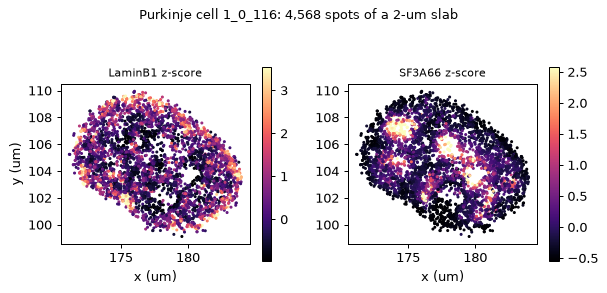
Because the signals and the coordinates are aligned spot by spot, the nuclear layout should show up in them: lamina-associated chromatin (LaminB1) at the nuclear edge, nuclear speckles (SF3A66) and active chromatin (H3K27ac) inside. Rank-correlate each mark with the spot’s distance from its nucleus centre (normalised per cell):

cell_of = cd.spots["cell_id"].astype(str).to_numpy()
xyz = np.asarray(cd.coords)
centre = pd.DataFrame(xyz, columns=list("xyz")).groupby(cell_of).transform("median").to_numpy()
r = np.linalg.norm(xyz - centre, axis=1)
r_norm = r / pd.Series(r).groupby(cell_of).transform(lambda s: s.quantile(0.95)).to_numpy()
rho = pd.Series({m: spearmanr(r_norm, tracks[m]).statistic
                 for m in ["LaminB1", "H3K9me3", "MajSat", "Fibrillarin", "H3K27ac", "SF3A66", "n_rad_score"]})
print("Spearman rho with the radial position:")
print(rho.round(3).to_string())

Spearman rho with the radial position:
LaminB1        0.116
H3K9me3       -0.129
MajSat        -0.018
Fibrillarin   -0.206
H3K27ac       -0.274
SF3A66        -0.343
n_rad_score    0.742

cell_id = cd.cells.index[cd.cells["cell_type"] == "Purkinje"][0]
one = cd.get_cell(cell_id)
mid = np.abs(one.coords[:, 2] - np.median(one.coords[:, 2])) < 1.0      # a 2-um optical slab
fig, axes = plt.subplots(1, 2, figsize=(7, 3.3))
for ax, mark in zip(axes, ["LaminB1", "SF3A66"]):
    v = one.spot_tracks[mark].to_numpy()[mid]
    sc = ax.scatter(one.coords[mid, 0], one.coords[mid, 1], c=v, s=2, cmap="magma",
                    vmin=np.percentile(v, 2), vmax=np.percentile(v, 98))
    ax.set_aspect("equal"); ax.set_title(f"{mark} z-score", fontsize=9)
    ax.set_xlabel("x (um)"); fig.colorbar(sc, ax=ax, shrink=0.8)
axes[0].set_ylabel("y (um)")
fig.suptitle(f"Purkinje cell {cell_id}: {mid.sum():,} spots of a 2-um slab", fontsize=10)
plt.tight_layout(); plt.show()

Cells, positions and embeddings (cells, cellm)

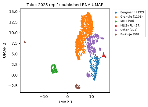
The clustering table gives each cell its leiden cluster, a cell type (through uns['leiden_to_cell_type']), nuclear volume and centroid. The centroid is stored in voxels with the voxel size in its uns['cell_spatial'] record, so cell_positions(physical=True) returns µm in the frame of coords (one frame per FOV, region = "{rep}_{fov}"). The published RNA UMAP is cellm['umap'].

print(cd.cells["cell_type"].value_counts().to_dict())
pos = cd.cell_positions(physical=True)
print({k: pos.attrs["cell_spatial"][k] for k in ("unit", "voxel_size", "frame", "region_col", "status")})
spot_centre = pd.DataFrame(xyz, columns=list("xyz")).groupby(cell_of).median().loc[pos.index]
offset = np.linalg.norm(spot_centre.to_numpy() - pos[["x", "y", "z"]].to_numpy(), axis=1)
print(f"centroid vs median DNA-spot position: median {np.median(offset):.2f} um, max {offset.max():.2f} um")
print("cellm:", {k: v.shape for k, v in cd.cellm.items()})
cd.cells.head()

{'Granule': 22, 'Other': 9, 'Bergmann': 8, 'MLI1': 3, 'Purkinje': 3, 'MLI2+PLI': 2}
{'unit': 'um', 'voxel_size': [0.103, 0.103, 0.25], 'frame': 'fov', 'region_col': 'fov', 'status': 'measured'}

centroid vs median DNA-spot position: median 0.62 um, max 1.96 um
cellm: {'umap': (47, 2)}

	leiden	cell_type	fov	centroid_x	centroid_y	centroid_z	nuc_volume_um3	doublet	batch
cell_id
1_0_72	0	Granule	1_0	1255.603	1677.512	13.784	117.001	0	1
1_0_104	0	Granule	1_0	1724.202	1535.181	14.662	120.823	0	1
1_0_123	0	Granule	1_0	876.227	1409.527	18.072	198.996	0	1
1_0_139	0	Granule	1_0	1823.625	1291.029	17.587	188.803	0	1
1_0_169	0	Granule	1_0	1635.217	1531.118	16.907	147.417	0	1

Per-cell summaries of the spot signals go to cells with uchrom.emb.aggregate_tracks (here the mean z-score of each IF channel, as if.<mark> columns).

marks = [m for m in IF_COLUMNS if m in tracks.columns]
aggregate_tracks(cd, marks, prefix="if", stat="mean")
summary = cd.cells.groupby("cell_type")[["if.H3K27ac", "if.H3K9me3", "if.H3K27me3", "if.LaminB1", "if.SF3A66"]].mean()
summary.insert(0, "n_cells", cd.cells["cell_type"].value_counts())
summary.round(2)

	n_cells	if.H3K27ac	if.H3K9me3	if.H3K27me3	if.LaminB1	if.SF3A66
cell_type
Bergmann	8	0.37	0.38	0.26	0.35	0.12
Granule	22	0.16	0.25	0.22	0.19	0.07
MLI1	3	0.34	0.44	0.43	0.29	0.08
MLI2+PLI	2	0.18	0.31	0.29	0.26	0.08
Other	9	0.23	0.30	0.24	0.29	0.09
Purkinje	3	0.44	0.38	0.72	0.35	0.02

Traces and the allele caveat (traces)

Homolog assignment is the weak point of this data. The loader builds traces from the highest-recall column dbscan_ldp_nbr_allele (the one the authors’ notebooks use) and records per-trace quality: n_loci, n_duplicate_loci (spots whose locus already occurs in the trace — more than 0 means two homologs or stray spots were merged) and how well the other two allele calls agree. If your analysis needs one fibre per trace (distance maps, TAD / loop calling), import with allele_col="dbscan_ldp_allele": fewer spots, no duplicates.

tr = cd.traces
print(f"dbscan_ldp_nbr_allele: {cd.n_spots:,} spots, {cd.n_traces:,} traces, "
      f"{(tr['n_duplicate_loci'] > 0).mean():.0%} of traces observe some locus twice")
strict = read_seqfish_multiomics(SPOTS, locus_annotation=LOCI, cell_clustering=CLUSTERS,
                                 allele_col="dbscan_ldp_allele")
print(f"dbscan_ldp_allele    : {strict.n_spots:,} spots ({strict.n_spots / cd.n_spots:.0%}), "
      f"{strict.n_traces:,} traces, {(strict.traces['n_duplicate_loci'] > 0).mean():.0%} with a repeated locus")
tr.head()

dbscan_ldp_nbr_allele: 383,674 spots, 1,500 traces, 85% of traces observe some locus twice

dbscan_ldp_allele    : 212,770 spots (55%), 1,432 traces, 0% with a repeated locus

	allele	n_spots	n_loci	n_duplicate_loci	dbscan_allele_majority	dbscan_allele_agreement	dbscan_ldp_allele_majority	dbscan_ldp_allele_agreement
trace_id
1_0_270_chr10_a1	1	818	754	64	1	1.000000	-1	0.564792
1_0_270_chr5_a1	1	696	654	42	1	1.000000	-1	0.547414
1_0_270_chrX_a1	1	980	893	87	1	0.997959	1	0.548980
1_0_270_chr14_a1	1	641	604	37	1	1.000000	-1	0.533541
1_0_270_chr17_a1	1	540	500	40	1	1.000000	-1	0.711111

{k: v for k, v in cd.uns.items() if k != "cell_spatial"}

{'genome_assembly': 'mm10',
 'xyz_unit': 'um',
 'voxel_xy_nm': 103,
 'voxel_z_nm': 250,
 'source': 'Takei2025_cerebellum',
 'zenodo_record': '7693825',
 'leiden_to_cell_type': {'0': 'Granule',
  '1': 'Granule',
  '2': 'Bergmann',
  '4': 'MLI1',
  '6': 'Purkinje',
  '11': 'Purkinje',
  '7': 'MLI2+PLI'},
 'allele_col': 'dbscan_ldp_nbr_allele',
 'keep_unclustered': False}

4. Streaming import into a store

With out=, read_seqfish_multiomics reads the FOV files one at a time into a .chromdata.zarr store, so memory holds one FOV (a full FOV CSV is 2–3 GB) instead of all of them, and returns the store opened backed. The store holds the same spots and signals as the in-memory import.

t0 = time.perf_counter()
store = read_seqfish_multiomics(SPOTS, locus_annotation=LOCI, cell_clustering=CLUSTERS,
                                out=OUT / "takei2025_fov0_47cells.chromdata.zarr")
print(f"streamed in {time.perf_counter() - t0:.1f} s -> {type(store).__name__}")


def table(x):
    """Spots + coordinates + per-spot signals, in a canonical row order."""
    df = pd.concat([x.to_dataframe().reset_index(drop=True), x.spot_tracks.reset_index(drop=True)], axis=1)
    df["trace_id"] = df["trace_id"].astype(str); df["cell_id"] = df["cell_id"].astype(str)
    return df.sort_values(["trace_id", "start", "x", "y", "z"]).reset_index(drop=True)


pd.testing.assert_frame_equal(table(cd), table(store.to_memory()), check_categorical=False)
pd.testing.assert_frame_equal(cd.cells.drop(columns=[c for c in cd.cells if c.startswith("if.")]), store.cells)
print(f"streamed store == in-memory import: {store.n_spots:,} spots x {store.spot_tracks.shape[1]} signals, "
      f"{len(store.cells)} cells")

streamed in 7.5 s -> BackedChromData

streamed store == in-memory import: 383,674 spots x 62 signals, 47 cells

5. The whole replicate, opened backed

Replicate 1 has three FOVs: 1,799 cells and 10.9 million spots (2 GB as a store). The public U-Chrom atlas holds it as a store (built by apps/atlas/recipes/build_takei2025_cerebellum.py from the Zenodo tarball), and ds.atlas("takei2025_cerebellum") opens it over HTTP, backed: the small tables load at once, spots are read only when asked for — here the spots of one Purkinje cell. uchrom.io.load_takei2025_cerebellum() is the local alternative: it downloads the 2.85 GB tarball and the RNA data from Zenodo, builds the store and the linked RNA AnnData in the data directory, and returns the data in memory (≈10 GB).

t0 = time.perf_counter()
rep1 = ds.atlas("takei2025_cerebellum")
print(f"opened in {time.perf_counter() - t0:.2f} s: {rep1.n_spots:,} spots, {rep1.n_traces:,} traces, "
      f"{rep1.n_cells:,} cells, {rep1.n_bins:,} loci, {len(rep1.spot_tracks.columns)} spot tracks")
print(rep1.cells["cell_type"].value_counts().to_dict())

t0 = time.perf_counter()
purk = rep1.get_cell(rep1.cells.index[rep1.cells["cell_type"] == "Purkinje"][0])
print(f"get_cell: {purk.n_spots:,} spots + {purk.spot_tracks.shape[1]} signals read in "
      f"{time.perf_counter() - t0:.2f} s")

umap, ctype = rep1.cellm["umap"], rep1.cells["cell_type"].astype(str).to_numpy()
fig, ax = plt.subplots(figsize=(5.5, 4))
for t in sorted(set(ctype)):
    m = ctype == t
    ax.scatter(umap[m, 0], umap[m, 1], s=4, label=f"{t} ({m.sum()})")
ax.set_xlabel("UMAP 1"); ax.set_ylabel("UMAP 2"); ax.set_title("Takei 2025 rep 1: published RNA UMAP", fontsize=10)
ax.legend(fontsize=7, markerscale=2, loc="upper left", bbox_to_anchor=(1.01, 1))
plt.tight_layout(); plt.show()

opened in 1.83 s: 10,912,638 spots, 59,112 traces, 1,799 cells, 100,049 loci, 62 spot tracks
{'Granule': 1109, 'Other': 323, 'Bergmann': 192, 'MLI1': 90, 'Purkinje': 58, 'MLI2+PLI': 27}

get_cell: 4,225 spots + 62 signals read in 1.26 s

Next steps

• chromdata_basics.ipynb — the container itself (backed stores, iter_cells, results).

• import_fofct.ipynb / import_pyhim_ecsv.ipynb — other imaging formats.

• Structure calling on imaging traces: tad_calling.ipynb, loop_calling.ipynb, compartment.ipynb (prefer allele_col="dbscan_ldp_allele" here).

• takei2025_auto_discovery.ipynb — LLM-driven hypothesis generation on this dataset.

• Browse the store: python -m uchrom_browser tutorials/_out/takei2025_fov0_47cells.chromdata.zarr.