ChromData: the data model

ChromData is the one object every U-Chrom module reads and writes: cells › traces › spots, each spot a 3-D position of one genomic locus, all spots pointing into one shared locus axis (bins). This tutorial walks through the format 2.x model on a real chromatin-tracing dataset: how to build an object, the locus axis, per-locus vs per-spot signals, the cell and trace tables, typed interval tables, results with provenance, subsetting, on-demand distances and cell positions.

Modules: chromdata (ChromData, chromdata.intervals, chromdata.results); one call to uchrom (uc.tl.call_tads) shows how analysis functions fill intervals and results. Data: Takei et al. 2021, Nature 590:344 (DNA seqFISH+, 201 mouse ES cells, 20 chromosomes × 60 loci of 25 kb), 4DN FOF-CT core table 4DNFIHF3JCBY.csv with its cell table 4DNFIFINA2U9.csv and nascent-RNA spot table 4DNFIJ52NVDV.csv; ds.fetch("takei") and ds.fetch("takei_tables") download them once from the 4DN data portal. Runtime: about 15 s. Storage on disk (.chromdata.zarr, backed reads, linked contact maps, the atlas) is the subject of chromdata_stores.

import itertools
import time
import warnings
from pathlib import Path

import matplotlib.pyplot as plt
import numpy as np
import pandas as pd

import chromdata
from chromdata import ChromData
import uchrom.datasets as ds

plt.rcParams["figure.dpi"] = 90

OUT = Path("_out") / "chromdata_basics"; OUT.mkdir(parents=True, exist_ok=True)   # tutorials/_out/ (ignored by git)

CORE = ds.fetch("takei")             # FOF-CT core table (4DN, 22 MB; downloaded once)
T = ds.fetch("takei_tables")         # its companion tables (4DN, 0.3 MB)
CELLS = T / "4DNFIFINA2U9.csv"       # FOF-CT cell table
RNA = T / "4DNFIJ52NVDV.csv"         # FOF-CT nascent-RNA spot table
print("chromdata", chromdata.__version__, "| data:", [p.relative_to(ds.data_dir()).as_posix() for p in (CORE, CELLS, RNA)])

chromdata 0.1.0 | data: ['4DNFIHF3JCBY.csv', '4DNFIFINA2U9.csv', '4DNFIJ52NVDV.csv']

The model at a glance

axis	one row per	attributes
spots	detected locus of one trace	coords (n_spots × 3), spots (bin_id, trace_id, cell_id, …), spot_tracks, layers
bins	locus, shared by all cells	bins (chrom, start, end), bin_tracks, binm, intervals
cells	cell	cells (incl. cell positions), cellm, cell_shapes, points (RNA spots, …)
traces	chromatin fibre (one homolog of one chromosome)	traces
–	analysis output	results (with provenance), uns

Pairwise distance matrices are never stored (they are per trace and O(n²)); contact maps and RNA matrices stay in their own files and are linked (see chromdata_stores).

Building a ChromData from a spot table

The minimum is coords (n_spots × 3) and a spots table with trace_id and either the loci (chrom, start, end) — the locus axis bins is then derived — or a bin_id into a bins table you pass. Here we read the spots of the first cell straight from the FOF-CT core table with pandas (the ##columns= header line names the columns) and build the object by hand.

with open(CORE) as fh:
    header = list(itertools.takewhile(lambda line: line.lstrip('"').startswith("#"), fh))
names = next(l for l in header if l.startswith("##columns=")).split("=", 1)[1].strip().strip(",").strip("()").split(",")
print(len(header), "header lines; columns:", names)

table = pd.read_csv(CORE, skiprows=len(header), header=None, names=names, nrows=3000)
one = table[table["Cell_ID"] == "0_1"]
spots = pd.DataFrame({"chrom": one["Chrom"], "start": one["Chrom_Start"], "end": one["Chrom_End"],
                      "trace_id": one["Trace_ID"], "cell_id": one["Cell_ID"], "spot_id": one["Spot_ID"]})
mini = ChromData(one[["X", "Y", "Z"]].to_numpy(), spots, uns={"genome_assembly": "mm10", "xyz_unit": "micron"})
mini

15 header lines; columns: ['Spot_ID', 'Trace_ID', 'X', 'Y', 'Z', 'Chrom', 'Chrom_Start', 'Chrom_End', 'Cell_ID', 'Extra_Cell_ROI_ID']

ChromData: n_spots=1473, n_traces=39, n_cells=1, n_bins=953
  spots:   ['chrom', 'start', 'end', 'trace_id', 'cell_id', 'spot_id', 'bin_id']
  uns:     ['genome_assembly', 'xyz_unit']

The constructor derived bins from the distinct loci (sorted by chromosome, start, end) and gave every spot a bin_id. Two spots of different homologs (traces …_0 and …_1) at the same locus share a bin:

display(mini.bins.head(3))
mini.spots.head(3)

	chrom	start	end
bin_id
0	chr1	135625000	135650000
1	chr1	135650000	135675000
2	chr1	135700000	135725000

	chrom	start	end	trace_id	cell_id	spot_id	bin_id
0	chr1	135625000	135650000	0_1_1_0	0_1	705144	0
1	chr1	135650000	135675000	0_1_1_0	0_1	705145	1
2	chr1	135650000	135675000	0_1_1_1	0_1	705146	1

The same object can be built from bin_id + bins=; chrom / start / end are then filled in from bins. Pass bins= whenever objects must share one locus axis — this cell alone saw only 953 of the 1,200 imaged loci. Missing required columns fail at construction:

mini2 = ChromData(mini.coords, mini.spots[["bin_id", "trace_id", "cell_id", "spot_id"]], bins=mini.bins)
print("same spots:", mini2.spots_with_loci()[mini.spots.columns].equals(mini.spots))
try:
    ChromData(mini.coords, spots.drop(columns="trace_id"))
except ValueError as err:
    print("ValueError:", err)

same spots: True
ValueError: spots missing required column: 'trace_id'

Loading the whole dataset with from_fofct

ChromData.from_fofct reads the core table and, optionally, its companion tables: the cell table becomes cells (cell-table centroids are registered as cell positions) and the RNA spot table becomes points["rna"]. The ## header lines go to uns.

t0 = time.perf_counter()
cd = ChromData.from_fofct(CORE, cell_table=CELLS, rna_table=RNA)
print(f"read in {time.perf_counter() - t0:.2f} s")
print(cd.n_cells, "cells,", cd.n_traces, "traces,", cd.n_spots, "spots,", cd.n_bins, "bins on", len(cd.chroms), "chromosomes")
print("uns:", {k: cd.uns[k] for k in ("genome_assembly", "xyz_unit")}, "+", [k for k in cd.uns if k not in ("genome_assembly", "xyz_unit")])

read in 0.46 s
201 cells, 8285 traces, 316995 spots, 1200 bins on 20 chromosomes
uns: {'genome_assembly': 'GRCm38/mm10', 'xyz_unit': 'micron'} + ['fofct_header', 'fofct_companions', 'cell_spatial']

A trace here is one homolog of one chromosome in one cell (Trace_ID = <fov>_<cell>_<chromosome>_<homolog>). Spots per trace and traces per cell:

per_trace = cd.spots.groupby("trace_id", observed=True).size()
per_cell = cd.spots.groupby("cell_id", observed=True)["trace_id"].nunique()
dup = cd.spots.duplicated(["trace_id", "bin_id"]).sum()
print(f"spots per trace: median {per_trace.median():.0f} of 60 loci (range {per_trace.min()}-{per_trace.max()})")
print(f"traces per cell: median {per_cell.median():.0f} (2 homologs x 20 chromosomes = 40)")
print(f"{dup:,} spots ({dup / cd.n_spots:.0%}) repeat a locus already detected in the same trace")

spots per trace: median 39 of 60 loci (range 1-154)
traces per cell: median 41 (2 homologs x 20 chromosomes = 40)
35,432 spots (11%) repeat a locus already detected in the same trace

The locus axis: bins and spots.bin_id

bins has one row per locus (index bin_id), shared by every cell; each spot points at one bin. The chrom / start / end columns of spots are derived from bins (they are not stored on disk); spots_with_loci() is the stable way to get them. chrom, trace_id and cell_id are categoricals.

display(cd.bins.groupby("chrom", observed=True).size().describe()[["count", "min", "max"]].rename("loci per chromosome").to_frame().T)
print({c: f"category ({len(t.categories)} values)" if isinstance(t, pd.CategoricalDtype) else str(t)
       for c, t in cd.spots.dtypes.items()})
as_object = cd.spots.astype({c: object for c in ("chrom", "trace_id", "cell_id")})
print(f"spots table: {cd.spots.memory_usage(deep=True).sum() / 1e6:.1f} MB with categoricals, "
      f"{as_object.memory_usage(deep=True).sum() / 1e6:.1f} MB with Python strings")

	count	min	max
loci per chromosome	20.0	60.0	60.0

{'chrom': 'category (20 values)', 'start': 'int64', 'end': 'int64', 'trace_id': 'category (8285 values)', 'spot_id': 'int64', 'cell_id': 'category (201 values)', 'extra_cell_roi_id': 'int64', 'bin_id': 'int64'}
spots table: 14.4 MB with categoricals, 64.6 MB with Python strings

To change loci, edit cd.bins (or edit the spot loci and call cd.rebuild_bins()); the derived spot columns cannot disagree with bins — the constructor checks it.

Per-locus and per-spot signals: bin_tracks, spot_tracks, binm

A value that belongs to a locus (bulk ChIP, GC content, a detection rate) is a column of bin_tracks (n_bins rows); a value measured on one spot (IF intensity, a per-spot distance) is a column of spot_tracks (n_spots rows). Two real examples: the fraction of traces in which each locus was detected, and each spot’s distance to the centre of its trace.

chrom_of_bin = cd.bins["chrom"].astype(str)
traces_per_chrom = cd.spots.groupby("chrom", observed=True)["trace_id"].nunique()
traces_per_bin = cd.spots.groupby("bin_id")["trace_id"].nunique().reindex(range(cd.n_bins), fill_value=0)
cd.bin_tracks["detection_rate"] = traces_per_bin.to_numpy() / chrom_of_bin.map(traces_per_chrom).to_numpy()

trace_code = cd.spots["trace_id"].cat.codes.to_numpy()
centre = pd.DataFrame(cd.coords).groupby(trace_code).transform("mean").to_numpy()
cd.spot_tracks["dist_to_trace_centre_um"] = np.linalg.norm(cd.coords - centre, axis=1)

print(cd.track_names())
print(f"detection rate per locus: median {cd.bin_tracks['detection_rate'].median():.2f} "
      f"(range {cd.bin_tracks['detection_rate'].min():.2f}-{cd.bin_tracks['detection_rate'].max():.2f})")
cd.tracks_spot_view().head(3)

{'bin': ['detection_rate'], 'spot': ['dist_to_trace_centre_um']}
detection rate per locus: median 0.57 (range 0.01-0.80)

	detection_rate	dist_to_trace_centre_um
0	0.438679	0.465144
1	0.431604	0.496312
2	0.431604	0.783389

tracks_spot_view() broadcasts the bin tracks to the spots (through bin_id) next to the spot tracks — the view analysis code often wants. (The 1.x attribute cd.tracks is a deprecated alias of that view; new code uses bin_tracks / spot_tracks.)

binm holds per-locus arrays with more than one value per bin. Each chromosome here has 60 loci, so the population median distance map of a chromosome fits as rows of a (n_bins, 60) array: row i holds the median distance of locus i to every locus of its chromosome (spots of the same locus in a trace are averaged first).

def median_distance_map(sub, bin_ids):
    # population median distance (um) between the loci bin_ids of one chromosome
    local = np.searchsorted(bin_ids, sub.spots["bin_id"].to_numpy())
    t = sub.spots["trace_id"].cat.remove_unused_categories().cat.codes.to_numpy()
    pos = np.zeros((t.max() + 1, len(bin_ids), 3)); n = np.zeros((t.max() + 1, len(bin_ids)))
    np.add.at(pos, (t, local), sub.coords); np.add.at(n, (t, local), 1)
    with warnings.catch_warnings():
        warnings.simplefilter("ignore", RuntimeWarning)    # loci a trace missed / pairs never seen: NaN
        pos /= n[..., None]
        d = np.linalg.norm(pos[:, :, None] - pos[:, None, :], axis=-1)
        return np.nanmedian(d, axis=0)

t0 = time.perf_counter()
med = np.full((cd.n_bins, 60), np.nan)
for chrom in cd.chroms:
    ids = np.flatnonzero(chrom_of_bin.to_numpy() == chrom)
    med[ids] = median_distance_map(cd.get_chrom(chrom), ids)
cd.binm["median_distance_um"] = med
print(f"binm['median_distance_um'] {med.shape} in {time.perf_counter() - t0:.1f} s; "
      f"neighbouring loci (25 kb apart): median {np.nanmedian(np.diagonal(med.reshape(20, 60, 60), 1, 1, 2)):.2f} um")

binm['median_distance_um'] (1200, 60) in 2.1 s; neighbouring loci (25 kb apart): median 0.18 um

Cells, traces, layers and points

cells is indexed by cell_id; here it holds the cell table (nucleus area, mRNA counts per gene as rna.<gene>, the authors’ QC flag keep1). cellm holds per-cell arrays whose rows follow cells — e.g. a PCA of the log-normalised mRNA counts:

genes = [c for c in cd.cells.columns if c.startswith("rna.")]
counts = cd.cells[genes].to_numpy(float)
logx = np.log1p(counts / counts.sum(1, keepdims=True) * 1e4)
u, s, _ = np.linalg.svd(logx - logx.mean(0), full_matrices=False)
cd.cellm["rna_pca"] = u[:, :10] * s[:10]
print(f"{len(genes)} genes; cellm:", {k: v.shape for k, v in cd.cellm.items()},
      f"; PC1-2 explain {(s[:2] ** 2).sum() / (s ** 2).sum():.0%} of the variance")
cd.cells[["keep1", "nucleus_area_um2", "rna.Nanog", "rna.Zfp42"]].head(3)

45 genes; cellm: {'rna_pca': (201, 10)} ; PC1-2 explain 35% of the variance

	keep1	nucleus_area_um2	rna.Nanog	rna.Zfp42
cell_id
0_1	0	242.161034	0.0	21.0
0_2	0	158.668204	1.0	95.0
0_3	0	203.735236	0.0	41.0

traces is the per-trace table, indexed by trace_id. We fill it from the data: chromosome, homolog (the last field of the id: 0 or 1 for most traces, -1, 2 or 3 for some, as deposited), number of spots and radius of gyration.

d2 = cd.spot_tracks["dist_to_trace_centre_um"].to_numpy() ** 2
g = pd.DataFrame({"trace_id": cd.spots["trace_id"].astype(str), "chrom": cd.spots["chrom"].astype(str), "d2": d2})
traces = g.groupby("trace_id").agg(chrom=("chrom", "first"), n_spots=("d2", "size"), rg_um=("d2", "mean"))
traces["rg_um"] = np.sqrt(traces["rg_um"])
traces["homolog"] = traces.index.str.rsplit("_", n=1).str[1].astype(int)
cd.traces = traces
print(cd.traces["homolog"].value_counts().to_dict())
cd.traces.head(3)

{0: 3987, 1: 3551, -1: 659, 2: 83, 3: 5}

	chrom	n_spots	rg_um	homolog
trace_id
0_10_10_0	chr10	33	0.499358	0
0_10_10_1	chr10	45	0.373785	1
0_10_11_0	chr11	50	0.336504	0

layers are alternative coordinate sets with the shape of coords (raw / drift-corrected / a second model). points are non-genomic 3-D points in the same frame, here the 3,335 nascent-RNA spots, linked to cells by cell_id.

cd.layers["trace_centred"] = cd.coords - centre
print({k: v.shape for k, v in cd.layers.items()})
print(len(cd.points["rna"]), "RNA spots; most frequent:", cd.points["rna"]["gene"].value_counts().head(3).to_dict())
cd.points["rna"][["x", "y", "z", "gene", "cell_id"]].head(3)

{'trace_centred': (316995, 3)}
3335 RNA spots; most frequent: {'Lgr4': 457, 'Actb': 454, 'Rpl5': 359}

	x	y	z	gene	cell_id
0	169.853	26.619	3.386	Auts2	0_1
1	152.599	24.696	2.371	Auts2	0_2
2	32.609	78.165	3.294	Auts2	0_10

Interval tables: intervals

cd.intervals maps a key to an IntervalTable, a DataFrame with a declared kind: domain (chrom, start, end: TADs, domains), pair (chrom1 … end2: loops), peak and segment (… label: compartments). Tables are validated when stored. The imaged regions make a small domain table:

regions = cd.bins.groupby("chrom", observed=True).agg(start=("start", "min"), end=("end", "max")).reset_index()
cd.intervals.add("regions.imaged", regions, kind="domain")
print(cd.intervals)
try:
    cd.intervals.add("broken", regions.assign(end=regions["start"] - 1), kind="domain")
except ValueError as err:
    print("ValueError:", err)
cd.intervals["regions.imaged"].head(3)

IntervalStore({'regions.imaged': <domain, 20 rows>})
ValueError: domain intervals must satisfy end >= start

	chrom	start	end
0	chr1	135600000	137100000
1	chr10	75400000	76900000
2	chr11	97425000	98925000

Results with provenance: results

cd.results is a ResultsStore: cd.results[key] is the value, cd.results.record(key) the value with its provenance (producing function, parameters, inputs, package version, time). Values must be storable (DataFrame / Series, numeric array, dict of those, JSON scalars); anything else fails at assignment, not at write().

long = cd.traces[cd.traces["n_spots"] >= 30]
rg = long.groupby("chrom")["rg_um"].median()
cd.results.set("rg.median_by_chrom", rg, function="tutorials/chromdata_basics.ipynb",
               params={"min_spots": 30}, inputs={"n_traces": len(long)})
print(cd.results)
print(cd.results.record("rg.median_by_chrom").provenance)
print(f"median Rg per chromosome (1.5 Mb regions): {rg.min():.2f}-{rg.max():.2f} um")
try:
    cd.results["not_storable"] = {1, 2, 3}
except TypeError as err:
    print("TypeError:", str(err)[:90], "...")

ResultsStore({'rg.median_by_chrom': <table>})
{'kind': 'table', 'function': 'tutorials/chromdata_basics.ipynb', 'params': {'min_spots': 30}, 'inputs': {'n_traces': 5815}, 'uchrom_version': '0.2.0', 'created_utc': '2026-10-06T22:52:45+00:00'}
median Rg per chromosome (1.5 Mb regions): 0.29-0.44 um
TypeError: results['not_storable']: cannot store a value of type set in cd.results. Supported: DataFr ...

Analysis functions of uchrom follow one convention: they store their table under key_added ("tads.arcfish" here) with provenance, and interval-like outputs also appear in cd.intervals (the same object, typed, with source_result pointing back to the record). ArcFISH TAD calling on chr3:

import uchrom as uc

t0 = time.perf_counter()
tads = uc.tl.call_tads(cd, chrom="chr3", device="cpu")
print(f"call_tads: {time.perf_counter() - t0:.1f} s, {len(tads)} domains over {tads['level'].nunique()} levels")
rec = cd.results.record("tads.arcfish")
print(cd.intervals)
print("kind:", cd.intervals["tads.arcfish"].kind, "| source_result:", cd.intervals["tads.arcfish"].source_result)
print("function:", rec.function, "| params:", rec.params)
tads[tads["level"] == 1]

call_tads: 2.3 s, 9 domains over 3 levels
IntervalStore({'regions.imaged': <domain, 20 rows>, 'tads.arcfish': <domain, 9 rows>})
kind: domain | source_result: tads.arcfish
function: uchrom.strc.tad.call_tads_by_pval | params: {'window_bp': 100000.0, 'fdr_cutoff': 0.1, 'hierarchical': True, 'max_levels': 4, 'prominence': 0.0, 'distance': 1, 'k_sigma': 4.0, 'frac': 0.1}

	chrom	start	end	level	score	pval	fdr
0	chr3	7675000	8550000	1	2.782943	0.001648	0.028022
1	chr3	8550000	8925000	1	2.782943	0.001648	0.028022
2	chr3	8925000	9050000	1	1.809940	0.015490	0.097475
3	chr3	9050000	9325000	1	1.764433	0.017202	0.097475

IntervalTable.to_bins projects intervals onto the locus axis — for example the level-1 domain of every chr3 locus as a bin track (-1 where no domain overlaps):

level1 = cd.intervals["tads.arcfish"].query("level == 1")
cd.bin_tracks["tad_chr3_level1"] = level1.to_bins(cd.bins, how="id").to_numpy()
cd.bin_tracks.loc[chrom_of_bin == "chr3", "tad_chr3_level1"].value_counts().sort_index().to_dict()

{0: 29, 1: 15, 2: 5, 3: 11}

Subsetting: get_cell, get_cells, get_trace, get_chrom, cd[rows]

Every subset is a new ChromData (the original is not modified). Cell- and trace-level tables follow the spots (cells, cellm, traces, points), the locus axis does not: bins and the per-locus data are kept whole, so subsets of one dataset always share one axis.

def summary(name, x):
    return {"subset": name, "n_spots": x.n_spots, "n_traces": x.n_traces, "n_cells": x.n_cells,
            "traces rows": len(x.traces), "rna points": len(x.points["rna"]),
            "n_bins": x.n_bins}

qc = cd.cells.index[cd.cells["keep1"] == 1]
subsets = {
    "cd": cd,
    'cd.get_cell("0_1")': cd.get_cell("0_1"),
    "cd.get_cells(keep1 == 1)": cd.get_cells(qc),
    'cd.get_trace("0_1_3_0")': cd.get_trace("0_1_3_0"),
    'cd.get_chrom("chr3")': cd.get_chrom("chr3"),
    "cd[dist to centre < 0.5 um]": cd[cd.spot_tracks["dist_to_trace_centre_um"].to_numpy() < 0.5],
    "cd[:1000]": cd[:1000],
}
pd.DataFrame([summary(k, v) for k, v in subsets.items()]).set_index("subset")

	n_spots	n_traces	n_cells	traces rows	rna points	n_bins
subset
cd	316995	8285	201	8285	3335	1200
cd.get_cell("0_1")	1473	39	1	39	2	1200
cd.get_cells(keep1 == 1)	256148	6293	151	6293	2890	1200
cd.get_trace("0_1_3_0")	40	1	1	1	2	1200
cd.get_chrom("chr3")	18150	408	201	408	3335	1200
cd[dist to centre < 0.5 um]	274318	8209	201	8209	3335	1200
cd[:1000]	1000	28	1	28	2	1200

columns= selects the spot-aligned columns to carry: columns="coords" keeps coordinates and the key columns only (on a backed store this decides what is read from disk, see chromdata_stores):

lean = cd.get_cell("0_1", columns="coords")
print("spots:", list(lean.spots.columns), "| spot tracks:", list(lean.spot_tracks.columns), "| layers:", list(lean.layers))

spots: ['chrom', 'start', 'end', 'trace_id', 'cell_id', 'bin_id'] | spot tracks: [] | layers: []

Distances on demand: compute_distances

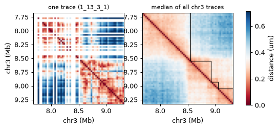
cd.compute_distances(trace_id=...) returns the pairwise distances of one trace’s spots. Below, the most complete chr3 trace without repeated loci, placed on the 60-locus grid, next to the population median map from binm with the level-1 ArcFISH domains.

chr3 = subsets['cd.get_chrom("chr3")']
stats = chr3.spots.groupby("trace_id", observed=True)["bin_id"].agg(["size", "nunique"])
tid = stats[stats["size"] == stats["nunique"]]["size"].idxmax()
d = cd.compute_distances(trace_id=tid)
ids = np.flatnonzero(chrom_of_bin.to_numpy() == "chr3")
local = np.searchsorted(ids, cd.get_trace(tid).spots["bin_id"].to_numpy())
single = np.full((60, 60), np.nan); single[np.ix_(local, local)] = d
print(f"trace {tid}: {d.shape[0]} spots, distance matrix {d.shape}")

mb = cd.bins.loc[ids, "start"].to_numpy() / 1e6
ext = [mb[0], mb[-1] + 0.025, mb[-1] + 0.025, mb[0]]
fig, axes = plt.subplots(1, 2, figsize=(7, 3.3))
for ax, m, title in [(axes[0], single, f"one trace ({tid})"), (axes[1], cd.binm["median_distance_um"][ids], "median of all chr3 traces")]:
    im = ax.imshow(m, cmap="RdBu", vmin=0, vmax=np.nanpercentile(cd.binm["median_distance_um"][ids], 98) * 1.3, extent=ext)
    ax.set_title(title, fontsize=9); ax.set_xlabel("chr3 (Mb)")
for _, r in level1.iterrows():
    a, b = r["start"] / 1e6, r["end"] / 1e6
    axes[1].plot([a, b, b], [a, a, b], color="k", lw=1)
axes[0].set_ylabel("chr3 (Mb)")
fig.colorbar(im, ax=axes, shrink=0.8, label="distance (um)")
plt.show()

trace 1_13_3_1: 46 spots, distance matrix (46, 46)

Cell positions: cell_positions, set_cell_positions

Where a cell sits is cell-level data: cells columns (centroid_x, centroid_y [, centroid_z]) plus a record in uns["cell_spatial"] that says what they are (unit, frame, measured or inferred, source). from_fofct registered the cell-table centroids:

pos = cd.cell_positions()
print(pos.attrs["cell_spatial"])
pos.head(3)

{'x_col': 'centroid_x', 'y_col': 'centroid_y', 'ndim': 2, 'status': 'measured', 'unit': 'micron', 'source': 'FOF-CT cell table Cent_ROI_x / Cent_ROI_y [/ Cent_ROI_z]'}

	x	y
cell_id
0_1	170.079	18.531
0_2	155.510	26.151
0_3	25.481	34.890

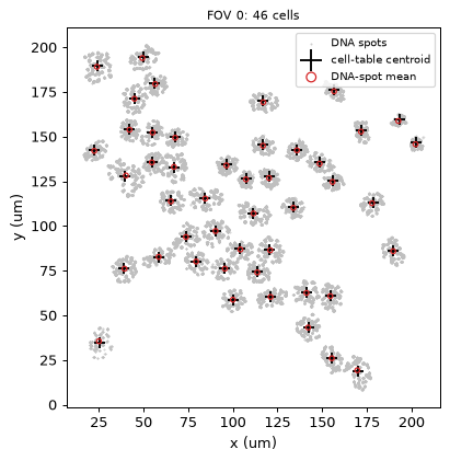
The record does not say yet which frame the centroids are in. The DNA spots give an independent estimate — the mean of each cell’s spots — which we store as a second position set (3-D, inferred, with its source). Cell ids start with the field of view, so positions are local to a FOV (region_col="fov").

cd.cells["fov"] = cd.cells.index.str.split("_").str[0]
spot_mean = pd.DataFrame(cd.coords, columns=["x", "y", "z"]).groupby(cd.spots["cell_id"].astype(str).to_numpy()).mean()
cd.set_cell_positions(spot_mean, key="dna_mean", unit="micron", frame="fov", region_col="fov",
                      in_coords_frame=True, status="inferred", source="mean of the cell's DNA seqFISH+ spots",
                      method="mean")
both = cd.cell_positions().join(cd.cell_positions("dna_mean"), rsuffix="_dna")
offset = np.hypot(both["x"] - both["x_dna"], both["y"] - both["y_dna"])
radius = np.sqrt(cd.cells["nucleus_area_um2"] / np.pi)
print(f"cell-table centroid vs DNA-spot mean: median {offset.median():.2f} um (max {offset.max():.2f}); "
      f"nucleus radius median {radius.median():.1f} um")
print("position sets:", list(cd.uns["cell_spatial"]), "| new columns:", [c for c in cd.cells.columns if c.startswith("dna_mean")])

cell-table centroid vs DNA-spot mean: median 0.50 um (max 1.58); nucleus radius median 7.4 um
position sets: ['default', 'dna_mean'] | new columns: ['dna_mean_centroid_x', 'dna_mean_centroid_y', 'dna_mean_centroid_z']

The two agree to half a micron, well inside a nucleus, so the cell-table centroids share the frame of coords. Re-registering the existing columns records that (positions=None, columns=[...]):

cd.set_cell_positions(columns=["centroid_x", "centroid_y"], unit="micron", frame="fov", region_col="fov",
                      in_coords_frame=True, source="FOF-CT cell table Cent_ROI_x / Cent_ROI_y")
print(cd.cell_positions().attrs["cell_spatial"])

fov0 = cd.cells.index[cd.cells["fov"] == "0"]
sub = cd.get_cells(fov0)
fig, ax = plt.subplots(figsize=(5, 5))
ax.scatter(sub.coords[:, 0], sub.coords[:, 1], s=0.05, c="0.75", rasterized=True, label="DNA spots")
p = cd.cell_positions().loc[fov0]; q = cd.cell_positions("dna_mean").loc[fov0]
ax.scatter(p["x"], p["y"], marker="+", s=60, c="k", label="cell-table centroid")
ax.scatter(q["x"], q["y"], s=12, facecolors="none", edgecolors="C3", label="DNA-spot mean")
ax.set_aspect("equal"); ax.set_xlabel("x (um)"); ax.set_ylabel("y (um)")
ax.set_title(f"FOV 0: {len(fov0)} cells", fontsize=9); ax.legend(fontsize=8, markerscale=2, loc="upper right")
plt.show()

{'x_col': 'centroid_x', 'y_col': 'centroid_y', 'ndim': 2, 'unit': 'micron', 'frame': 'fov', 'region_col': 'fov', 'in_coords_frame': True, 'status': 'measured', 'source': 'FOF-CT cell table Cent_ROI_x / Cent_ROI_y'}

Export and a round trip

to_dataframe() gives the flat structure table (one row per spot: loci, x, y, z and the spot columns), to_anndata() the cell-level part (cells as obs, cellm as obsm), to_fofct() a FOF-CT table. write() keeps everything; reading the store back returns every piece added above.

display(cd.to_dataframe().head(3))
adata = cd.to_anndata()
print("to_anndata:", adata.shape, "obsm:", list(adata.obsm))

path = OUT / "takei2021_basics.chromdata.zarr"
cd.write(path)
back = ChromData.read(path)
checks = {
    "bin_tracks": back.bin_tracks.equals(cd.bin_tracks),
    "binm": np.array_equal(back.binm["median_distance_um"], cd.binm["median_distance_um"], equal_nan=True),
    "cellm": np.array_equal(back.cellm["rna_pca"], cd.cellm["rna_pca"]),
    "traces": back.traces.sort_index().equals(cd.traces.sort_index()),
    "intervals": sorted(back.intervals) == sorted(cd.intervals),
    "results + provenance": back.results.record("tads.arcfish").provenance == rec.provenance,
    "cell positions": back.cell_positions("dna_mean").equals(cd.cell_positions("dna_mean")),
    "spot tracks (sorted by spot_id)": np.allclose(
        back.spot_tracks["dist_to_trace_centre_um"].to_numpy()[np.argsort(back.spots["spot_id"].to_numpy())],
        cd.spot_tracks["dist_to_trace_centre_um"].to_numpy()[np.argsort(cd.spots["spot_id"].to_numpy())]),
}
print(path, checks)

	chrom	start	end	x	y	z	trace_id	spot_id	cell_id	extra_cell_roi_id
0	chr1	135625000	135650000	176.998	15.132	2.821	0_1_1_0	705144	0_1	0
1	chr1	135650000	135675000	176.953	15.056	2.771	0_1_1_0	705145	0_1	0
2	chr1	135650000	135675000	165.263	21.032	2.931	0_1_1_1	705146	0_1	0

to_anndata: (201, 0) obsm: ['rna_pca']

_out/chromdata_basics/takei2021_basics.chromdata.zarr {'bin_tracks': True, 'binm': True, 'cellm': True, 'traces': True, 'intervals': True, 'results + provenance': True, 'cell positions': True, 'spot tracks (sorted by spot_id)': True}

Next steps

• chromdata_stores — the .chromdata.zarr store: row order, backed reads of one cell or chromosome, streaming writes, linked contact maps and AnnData, embedded copies and the public atlas over HTTP.

• import_fofct — more on FOF-CT import and export.

• tad_calling, loop_calling, compartment — the structure callers that fill intervals and results.

• fish_imputation — filling in undetected loci (uchrom.pp.impute).