Bulk Hi-C to 3-D: MDS and IGM population deconvolution

A bulk Hi-C map averages millions of cells. This tutorial turns one into 3-D structures in two ways: a single consensus structure by multidimensional scaling (uchrom.recon.bulk.mds: contacts → distances → SMACOF, PyTorch on CPU / CUDA / Apple MPS), and a population of structures whose contacts together reproduce the map — IGM’s deconvolution (uchrom.recon.bulk.deconv.deconvolve(..., method="igm") on the native engine uchrom_recon). Both are checked against the input and against imaging data the methods never saw.

Data: Rao et al. 2014, Cell 159:1665 (in situ Hi-C, IMR90, GEO GSE63525), chromosome 21 at 5 kb, hg19 — ds.fetch("rao2014_imr90_chr21") builds it once (a 3.8 MB .cool, by HTTP range reads of the GEO .hic); for the independent check, Bintu et al. 2018, Science 362:eaau1783 (chromatin tracing of IMR90 chr21:20.0–21.95 Mb hg19, 30 kb segments) — ds.fetch("bintu_imr90") downloads it once (2 MB, GitHub). Runtime: about 3 min on a laptop CPU (18 cores), most of it the IGM population (50 structures).

import contextlib
import io
import subprocess
import sys
import time
import warnings
from pathlib import Path

import cooler
import matplotlib.pyplot as plt
import numpy as np
import pandas as pd
import torch
from scipy.spatial.distance import pdist, squareform
from scipy.stats import pearsonr, spearmanr

import uchrom.datasets as ds
from chromdata import ChromData
from uchrom.io import read_bintu_tracing
from uchrom.recon.bulk.deconv import deconvolve
from uchrom.recon.bulk.deconv.igm import contact_probabilities, population_array
from uchrom.recon.bulk.deconv.preprocess import IGMPreprocessParams, preprocess_hic
from uchrom.recon.bulk.mds import apply_transform, procrustes_alignment, run_mds

plt.rcParams["figure.dpi"] = 90
warnings.filterwarnings("ignore", message="linalg.eigh: matrix too large")   # MPS falls back to the CPU for the eigen-decomposition

OUT = Path("_out") / "bulk_reconstruction"; OUT.mkdir(parents=True, exist_ok=True)   # outputs: tutorials/_out/ (ignored by git)

COOL = ds.fetch("rao2014_imr90_chr21")   # Rao 2014 IMR90 chr21, 5 kb, raw counts, hg19 (built once from the GEO .hic)
BINTU = ds.fetch("bintu_imr90")          # Bintu 2018 IMR90 chr21 tracing (GitHub; downloaded once)
clr5 = cooler.Cooler(str(COOL))
print(f"{COOL.relative_to(ds.data_dir())}: {clr5.info['nbins']:,} bins x {clr5.binsize // 1000} kb, "
      f"{clr5.info['sum']:,} contacts ({clr5.info['genome-assembly']})")

rao2014_imr90/IMR90_chr21_5kb_hg19.cool: 9,626 bins x 5 kb, 10,266,877 contacts (hg19)

The input map

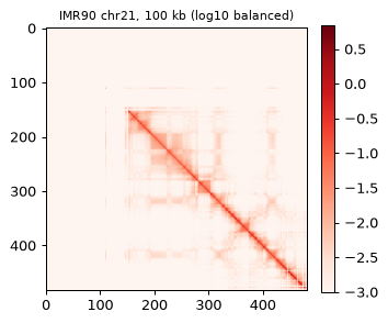
Whole-chromosome MDS works on a dense matrix, so we sum the 5 kb map into 100 kb bins (cooler.coarsen_cooler) and balance it (ICE, cooler.balance_cooler). The first ~14 Mb of chr21 (the acrocentric short arm) have no mappable reads.

def coarsened(res):
    path = OUT / f"IMR90_chr21_{res // 1000}kb.cool"
    if not path.exists():
        cooler.coarsen_cooler(str(COOL), str(path), factor=res // clr5.binsize, chunksize=10_000_000)
        cooler.balance_cooler(cooler.Cooler(str(path)), store=True)
    clr = cooler.Cooler(str(path))
    return path, clr.bins().fetch("chr21")[["chrom", "start", "end"]].reset_index(drop=True), \
        np.nan_to_num(clr.matrix(balance=True).fetch("chr21"))


COOL100, bins100, M100 = coarsened(100_000)
print(f"100 kb: {len(bins100)} bins, {(M100.sum(1) > 0).sum()} with contacts")
fig, ax = plt.subplots(figsize=(4, 3.6))
im = ax.imshow(np.log10(M100 + 1e-4), cmap="Reds", vmin=-3)
ax.set_title("IMR90 chr21, 100 kb (log10 balanced)", fontsize=9)
fig.colorbar(im, ax=ax, fraction=0.046)
fig.tight_layout()

100 kb: 482 bins, 327 with contacts

A consensus structure by MDS

run_mds drops bins without contacts, smooths the map with a distance-decay prior (weight, the share of the expected count mixed into every entry), converts contacts to distances d = c^(-1/alpha), and minimises the stress with SMACOF from a classical-MDS start (method="adam" uses autograd + Adam on the same stress instead). It returns the coordinates of the kept bins and the mask. The units are arbitrary (mean target distance 1).

t0 = time.time()
X100, keep100 = run_mds(torch.from_numpy(M100), alpha=4.0, weight=0.05, device="cpu", n_iter=1000)
t_mds = time.time() - t0
kept = bins100[keep100].reset_index(drop=True)
mds = ChromData.from_dataframe(kept.assign(x=X100[:, 0], y=X100[:, 1], z=X100[:, 2]), cell_id="IMR90_bulk",
                               uns={"xyz_unit": "arbitrary (MDS)", "genome_assembly": "hg19"})
mds.write(OUT / "IMR90_chr21_100kb_mds.chromdata.zarr")
print(f"SMACOF on the CPU: {t_mds:.2f} s -> {mds}")

Processing on device: cpu (dtype: torch.float64)
  Removed 155 zero-contact bins (327/482 kept)

SMACOF on the CPU: 0.34 s -> ChromData: n_spots=327, n_traces=1, n_cells=1, n_bins=327
  spots:   ['chrom', 'start', 'end', 'trace_id', 'cell_id', 'bin_id']
  uns:     ['xyz_unit', 'genome_assembly']

Quality checks

No single number says that a consensus structure is right. We use four:

1. Input–output correlation — Spearman correlation between the contact frequency and 1 / d over the observed pairs: does the structure reproduce the map?

2. The same after removing the distance decay (each value divided by the mean at its genomic separation): does it reproduce more than the polymer trend — domains, compartments?

3. Solver agreement — SMACOF vs Adam, Pearson r of pairwise distances after Procrustes superposition.

4. Imaging — the Bintu 2018 tracing of chr21:20.0–21.95 Mb in IMR90 cells, which MDS never saw: correlation between model distances and the median distances of 1,277 imaged chromosomes.

def observed_over_expected(A):
    # divide every off-diagonal entry by the mean of its diagonal (genomic separation)
    n = len(A); out = np.full_like(A, np.nan, dtype=float)
    for k in range(1, n):
        i = np.arange(n - k); v = A[i, i + k]; pos = v > 0
        if pos.any():
            out[i, i + k] = out[i + k, i] = np.where(pos, v / v[pos].mean(), np.nan)
    return out


def io_checks(X, M):
    D = squareform(pdist(X)); iu = np.triu_indices(len(X), 1)
    ok = M[iu] > 0
    rho = spearmanr(M[iu][ok], 1 / D[iu][ok])[0]
    Moe, Doe = observed_over_expected(M), observed_over_expected(D)
    ok2 = np.isfinite(Moe[iu]) & np.isfinite(Doe[iu])
    rho_oe = spearmanr(Moe[iu][ok2], 1 / Doe[iu][ok2])[0]
    return rho, rho_oe


fish = read_bintu_tracing(str(BINTU), chrom="chr21", start_bp=20_000_032, resolution_bp=30_000)
fish.uns["genome_assembly"] = "hg19"       # segment 1 at hg19 chr21:20,000,032 (= hg38 18,627,714)
fl = fish.spots_with_loci()
print(f"Bintu 2018: {fish.n_traces:,} imaged chromosomes x {fish.n_bins} segments, "
      f"chr21:{fl['start'].min():,}-{fl['end'].max():,} (hg19)")


def fish_on_bins(bins):
    # median FISH distance (nm) between model bins: segments averaged per bin and trace, then median over traces
    ends = bins["end"].to_numpy()
    b = np.searchsorted(ends, ((fl["start"] + fl["end"]) // 2).to_numpy(), side="right")
    cen = pd.DataFrame(fish.coords, columns=list("xyz")).assign(trace=fl["trace_id"].to_numpy(), bin=b) \
        .groupby(["trace", "bin"])[list("xyz")].mean()
    ub = np.sort(cen.index.get_level_values("bin").unique())
    C = np.full((cen.index.get_level_values("trace").nunique(), len(ub), 3), np.nan)
    C[pd.factorize(cen.index.get_level_values("trace"))[0], np.searchsorted(ub, cen.index.get_level_values("bin"))] = cen.to_numpy()
    with warnings.catch_warnings():                 # all-NaN pairs (bins not imaged in a trace)
        warnings.simplefilter("ignore", RuntimeWarning)
        D = np.nanmedian(np.linalg.norm(C[:, :, None] - C[:, None], axis=-1), axis=0)
    return ub, D, C


def fish_r(X, bins):
    ub, Df, _ = fish_on_bins(bins)
    Dm = squareform(pdist(X[ub])); iu = np.triu_indices(len(ub), 1)
    return pearsonr(Df[iu], Dm[iu])[0], len(ub)


rho, rho_oe = io_checks(X100, M100[keep100][:, keep100])
r_fish, n_fish = fish_r(X100, kept)
t0 = time.time()
with contextlib.redirect_stdout(io.StringIO()):          # run_mds reports the device and the dropped bins
    X_adam, _ = run_mds(torch.from_numpy(M100), alpha=4.0, weight=0.05, device="cpu", n_iter=1000, method="adam")
t_adam = time.time() - t0
R, t, s = procrustes_alignment(X_adam, X100)
r_solvers = pearsonr(pdist(apply_transform(X_adam, R, t, s)), pdist(X100))[0]
print(f"1. input-output Spearman (contact vs 1/d):         {rho:.3f}")
print(f"2. the same on observed/expected:                  {rho_oe:.3f}")
print(f"3. SMACOF ({t_mds:.2f} s) vs Adam ({t_adam:.2f} s), distance r: {r_solvers:.3f}")
print(f"4. vs Bintu FISH median distances ({n_fish} bins):  Pearson {r_fish:.3f}")

Bintu 2018: 1,277 imaged chromosomes x 65 segments, chr21:20,000,032-21,950,032 (hg19)

1. input-output Spearman (contact vs 1/d):         0.924
2. the same on observed/expected:                  0.803
3. SMACOF (0.34 s) vs Adam (1.98 s), distance r: 0.995
4. vs Bintu FISH median distances (20 bins):  Pearson 0.627

Resolution and device

Finer bins mean more, sparser bins: the map is noisier, MDS has more to place, and the agreement with the input drops. device="auto" takes CUDA or Apple MPS (float32) when available.

rows = []
for res in (250_000, 100_000, 50_000, 25_000):
    _, b, M = coarsened(res)
    for dev in ("cpu", "auto"):
        t0 = time.time()
        with contextlib.redirect_stdout(io.StringIO()):
            X, keep = run_mds(torch.from_numpy(M), alpha=4.0, weight=0.05, device=dev, n_iter=1000)
        dt = time.time() - t0
        rho, rho_oe = io_checks(X, M[keep][:, keep])
        rows.append({"resolution_kb": res // 1000, "device": dev, "bins_kept": int(keep.sum()), "seconds": dt,
                     "io_spearman": rho, "io_spearman_oe": rho_oe,
                     "fish_pearson": fish_r(X, b[keep].reset_index(drop=True))[0]})
sweep = pd.DataFrame(rows)
sweep.round(3)

	resolution_kb	device	bins_kept	seconds	io_spearman	io_spearman_oe	fish_pearson
0	250	cpu	127	0.060	0.944	0.836	0.861
1	250	auto	127	0.372	0.944	0.836	0.861
2	100	cpu	327	0.175	0.924	0.803	0.627
3	100	auto	327	0.223	0.924	0.803	0.627
4	50	cpu	660	0.542	0.867	0.722	0.578
5	50	auto	660	0.481	0.867	0.722	0.578
6	25	cpu	1321	0.656	0.738	0.568	0.641
7	25	auto	1321	0.511	0.738	0.568	0.641

At 100–250 kb the consensus structure reproduces the map, also beyond the distance decay (the O/E column); finer bins are sparser and the agreement drops. The imaged distances are matched only moderately (r ≈ 0.6 at 25–100 kb; the higher value at 250 kb rests on 8 bins and mostly reflects the distance decay): one consensus structure averages over very different single-cell conformations. device="auto" (Apple MPS here) gives the same structures; at these sizes (at most 1,321 bins, about a second) the device hardly matters — a GPU pays off for matrices of many thousands of bins.

Command line

python -m uchrom.recon.bulk.mds does the same from a .hic, .mcool or .cool file (balanced matrix; --partitioned for TAD-wise divide and conquer at high resolution, --inter for a whole-genome structure with inter-chromosomal contacts):

out = OUT / "IMR90_chr21_100kb_mds_cli.chromdata.zarr"
cmd = [sys.executable, "-m", "uchrom.recon.bulk.mds", str(COOL100), str(out),
       "--resolution=100000", "--chrom=chr21", "--device=cpu"]
run = subprocess.run(cmd, capture_output=True, text=True)
print("$ python", " ".join(cmd[1:]))
print(f"exit code {run.returncode}; {ChromData.read(out).n_spots} bins written to {out}")

$ python -m uchrom.recon.bulk.mds _out/bulk_reconstruction/IMR90_chr21_100kb.cool _out/bulk_reconstruction/IMR90_chr21_100kb_mds_cli.chromdata.zarr --resolution=100000 --chrom=chr21 --device=cpu
exit code 0; 327 bins written to _out/bulk_reconstruction/IMR90_chr21_100kb_mds_cli.chromdata.zarr

A population of structures: IGM

IGM (Boninsegna et al. 2022, Nat Methods 19:938; its predecessor PGS: Tjong et al. 2016, PNAS 113:E1663) fits a population of S diploid structures to the map. The map is first turned into contact probabilities; then IGM alternates an assignment step (A: given the current population, decide which structures should carry each contact so that the fraction of structures in contact matches its probability) and a modelling step (M: anneal and minimise every structure under its contacts, chain connectivity, excluded volume and the nuclear envelope), lowering a probability threshold σ from 1 to 0.01 so that rarer contacts enter step by step. The native engine runs both steps (protocol "igm", multi-core CPU or GPU); coordinates are in nm.

Hi-C → contact probabilities

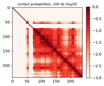
preprocess_hic implements the preprocessing of the IGM paper (Supplementary section 6): coverage filter and Knight–Ruiz balancing at 20 kb, then 200 kb probabilities from the top 10 % of the fine values of every block, with the scale chosen so that a bin has 24 contacts on average; neighbours get probability 1.

t0 = time.time()
prob = preprocess_hic(COOL, chroms=["chr21"], params=IGMPreprocessParams())   # 20 kb fine, 200 kb coarse
P = prob.probabilities.toarray()
pv = prob.provenance
print(f"{time.time() - t0:.1f} s: {pv['n_coarse']} bins of 200 kb, {pv['n_coarse_masked']} masked (no valid 20 kb bin); "
      f"f_max = {pv['fmax']:.2e}, mean contacts per bin {pv['average_contacts_final']:.1f}")
print("pairs with p >= sigma:", {s: v["intra"] for s, v in pv["pairs_at_or_above"].items()})
fig, ax = plt.subplots(figsize=(4, 3.6))
im = ax.imshow(np.log10(P + 1e-4), cmap="Reds", vmin=-3, vmax=0)
ax.set_title("contact probabilities, 200 kb (log10)", fontsize=9)
fig.colorbar(im, ax=ax, fraction=0.046)
fig.tight_layout()

0.7 s: 241 bins of 200 kb, 62 masked (no valid 20 kb bin); f_max = 3.39e-03, mean contacts per bin 24.0
pairs with p >= sigma: {'1.0': 521, '0.2': 2503, '0.1': 5575, '0.05': 9934, '0.02': 11913, '0.01': 12180}

Running the population

We model chr21 alone — both copies (ploidy="diploid", the default) — inside a full-size nucleus (sphere of 5 µm radius). occupancy_scope sets the bead size: with the diploid genome size (2 × 3.1 Gb) the beads get the size they have in a whole-genome model at 20 % occupancy (IGM’s default), instead of chr21 alone filling 20 % of the nucleus. IGM’s defaults are 10,000 structures (the paper: 1,000 at 200 kb); here 50 structures on the CPU keep the run to a few minutes — a small population, enough for the checks below. Use device="gpu" and thousands of structures for real work (out="pop.chromdata.zarr" streams a large population to disk).

N_STRUCTURES = 50
GENOME_BP = 2 * 3.1e9                     # diploid human genome: beads sized as in a whole-genome model
t0 = time.time()
rounds = []
pop = deconvolve(prob.probabilities, bins=prob.bins, method="igm", n_structures=N_STRUCTURES, device="cpu",
                 seed=1, occupancy_scope=GENOME_BP, progress=rounds.append)
t_igm = time.time() - t0
pop.write(OUT / "IMR90_chr21_igm.chromdata.zarr")
print(f"IGM: {N_STRUCTURES} structures in {t_igm / 60:.1f} min on the CPU ({pop.uns['deconv']['engine']})")
pop

IGM: 50 structures in 3.9 min on the CPU (cpu[18 threads])

ChromData: n_spots=24100, n_traces=100, n_cells=50, n_bins=241
  spots:   ['chrom', 'start', 'end', 'trace_id', 'cell_id', 'bin_id']
  cells:   ['violation_score', 'n_hic_restraints', 'hic_imposed', 'hic_violated', 'poly_imposed', 'poly_violated', 'env_imposed', 'env_violated', 'hic_inter_imposed', 'hic_inter_violated', 'energy', 'cg_iterations'] (50 cells)
  tracks (bins):  ['radius_nm', 'input_prob_rowsum']
  traces:  ['cell_id', 'chrom', 'copy'] (100 traces)
  results: ['deconv.igm']
  uns:     ['deconv', 'xyz_unit']

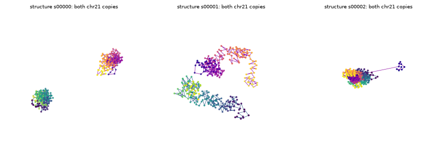
The population is a ChromData like any other: one cell per structure (s00000 …, with its violation statistics in cells), one trace per chromosome copy (s00000:chr21:0, traces has chrom / copy), one spot per bead; bin_tracks["radius_nm"] holds the bead radii and uns["deconv"] the parameters and the per-round log.

log = pd.DataFrame([{k: r[k] for k in ("round", "intra_sigma", "iteration", "n_pairs_restrained",
                                        "violation_score", "seconds_mstep")} for r in pop.uns["deconv"]["rounds"]])
print(f"bead radius {np.nanmedian(pop.bin_tracks['radius_nm']):.0f} nm; "
      f"structures with violations: {(pop.cells['violation_score'] > 0).sum()} of {len(pop.cells)} "
      f"(max violation score {pop.cells['violation_score'].max():.4f})")
log.round(4)

bead radius 93 nm; structures with violations: 19 of 50 (max violation score 0.0015)

	round	intra_sigma	iteration	n_pairs_restrained	violation_score	seconds_mstep
0	1	1.00	0	521	0.0000	17.9505
1	2	0.20	0	2499	0.0004	31.6068
2	3	0.10	0	5282	0.0005	54.3163
3	4	0.05	0	8664	0.0007	33.3752
4	5	0.02	0	9004	0.0004	32.7315
5	6	0.01	0	8611	0.0002	50.7969

Checks

1. Fit: the population’s contact probabilities (contact_probabilities: the fraction of structures and copies in which two beads touch, IGM’s own definition) against the input probabilities.

2. Imaging, never used by IGM: distances in nm against the Bintu 2018 medians in the same region — both the pattern (Pearson) and the absolute scale (model / FISH).

3. Cell-to-cell variability: a population should spread like single cells do. Compare the distribution of one distance across structures with the same distance across imaged chromosomes.

Pm = contact_probabilities(pop)
valid = ~prob.bins["masked"].to_numpy()
iu = np.triu_indices(len(P), 1)
m = valid[iu[0]] & valid[iu[1]]
x, y = P[iu][m], Pm[iu][m]
print(f"1. fit: Pearson {pearsonr(x, y)[0]:.3f} over {m.sum():,} pairs; "
      f"mean |p_model - p_input| {np.abs(x - y)[x >= 0.01].mean():.3f} for p >= 0.01")

X, pbins, cell_ids = population_array(pop)                 # (structures, bins, copies, 3), nm
ub, Df, C = fish_on_bins(pop.bins)
Y = X[:, ub]
Dpop = np.concatenate([np.linalg.norm(Y[:, :, k, None] - Y[:, None, :, k], axis=-1) for k in range(Y.shape[2])])
Dm = np.nanmedian(Dpop, axis=0)
iu2 = np.triu_indices(len(ub), 1)
print(f"2. vs FISH ({len(ub)} bins of 200 kb): Pearson {pearsonr(Df[iu2], Dm[iu2])[0]:.3f}, "
      f"median ratio model / FISH {np.median(Dm[iu2] / Df[iu2]):.2f}")

i, j = 0, len(ub) - 1
d_fish = np.linalg.norm(C[:, i] - C[:, j], axis=-1); d_fish = d_fish[np.isfinite(d_fish)]
d_pop = Dpop[:, i, j]
print(f"3. {pop.bins.loc[ub[i], 'start'] / 1e6:.1f} Mb <-> {pop.bins.loc[ub[j], 'start'] / 1e6:.1f} Mb: "
      f"coefficient of variation FISH {d_fish.std() / d_fish.mean():.2f}, IGM {d_pop.std() / d_pop.mean():.2f}")

fig, ax = plt.subplots(1, 3, figsize=(12, 3.3))
ax[0].scatter(x, y, s=2, alpha=0.3, color="0.3"); ax[0].plot([0, 1], [0, 1], "C3", lw=0.8)
ax[0].set_xlabel("input probability"); ax[0].set_ylabel("population probability"); ax[0].set_title("fit", fontsize=9)
ax[1].scatter(Df[iu2], Dm[iu2], s=10, color="0.3")
lim = [0, max(Df[iu2].max(), Dm[iu2].max()) * 1.05]; ax[1].plot(lim, lim, "C3", lw=0.8)
ax[1].set_xlabel("FISH median distance (nm)"); ax[1].set_ylabel("IGM median distance (nm)")
ax[1].set_title("held-out imaging", fontsize=9)
bins_h = np.linspace(0, np.percentile(np.r_[d_fish, d_pop], 99), 30)
ax[2].hist(d_fish, bins=bins_h, density=True, alpha=0.5, label="FISH (single chromosomes)")
ax[2].hist(d_pop, bins=bins_h, density=True, alpha=0.5, label="IGM (structures x copies)")
ax[2].set_xlabel("distance (nm)"); ax[2].legend(fontsize=7); ax[2].set_title("variability of one distance", fontsize=9)
fig.tight_layout()

1. fit: Pearson 0.989 over 15,931 pairs; mean |p_model - p_input| 0.024 for p >= 0.01

2. vs FISH (10 bins of 200 kb): Pearson 0.864, median ratio model / FISH 0.80
3. 20.0 Mb <-> 21.8 Mb: coefficient of variation FISH 0.68, IGM 0.28

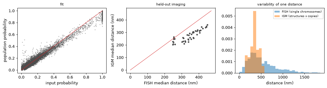
The population reproduces the input probabilities closely — that is what IGM optimises — and, without having seen the imaging, the pattern of the imaged distances and their absolute scale to within about 20 % (the model is somewhat more compact; its scale comes only from the nucleus size, the occupancy and the contact definition). It is less variable than the imaged chromosomes: part of the FISH spread is measurement noise (localisation error, missed segments), part is cell-to-cell heterogeneity that 50 structures fitted to a 200 kb map do not reach. Three of the structures — each holds two copies of chr21, often in separate territories:

from mpl_toolkits.mplot3d import Axes3D  # noqa: F401 (registers the 3-D projection)

fig = plt.figure(figsize=(10, 3.4))
for k in range(3):
    ax = fig.add_subplot(1, 3, k + 1, projection="3d")
    for cp, cmap in ((0, "viridis"), (1, "plasma")):
        Z = X[k, valid, cp]
        ax.plot(*Z.T, lw=0.6, color=plt.get_cmap(cmap)(0.3))
        ax.scatter(*Z.T, c=np.arange(len(Z)), cmap=cmap, s=4)
    ax.set_title(f"structure {cell_ids[k]}: both chr21 copies", fontsize=8); ax.set_axis_off()
fig.tight_layout()

Notes

• What the numbers mean: the MDS checks use the map the structure was computed from (1–3) and one held-out imaging region (4). The IGM fit is the quantity IGM optimises; the FISH comparison is independent of it — including the absolute scale, which comes only from the nucleus size and the bead packing.

• Population size: IGM’s statistics converge with thousands of structures (the IGM paper: 1,000 at 200 kb, whole genome). The native engine runs those on a GPU (device="gpu") or a multi-core CPU; benchmarks/bulk/ compares it with the original IGM.

• Whole genome: pass all chromosomes to preprocess_hic (and a .mcool / .hic); then inter-chromosomal probabilities enter the A-step as well, and occupancy_scope can stay "model".

• Citations: IGM — Boninsegna et al. 2022 (doi:10.1038/s41592-022-01527-x), PGS — Tjong et al. 2016, Hua et al. 2018 (uns["deconv"]["citations"]); MDS follows miniMDS (Rieber & Mahony 2017).

Next steps

• reconstruction — single-cell Hi-C to 3-D (NucDynamics, EMber).

• gem_fish_reconstruction — the same Hi-C together with the Bintu tracing as restraints (GEM-FISH).

• tad_calling, compartment — structure calling on 3-D data, including reconstructed populations.