A/B compartments from chromatin tracing
This tutorial calls A/B compartments from traces with
uchrom.strc.comp.call_compartments_axes_pc (also uc.tl.call_compartments),
an independent implementation of ArcFISH’s ABCaller.by_axes_pc (Yu et al.
2025, bioRxiv 10.1101/2025.11.26.690837). You will call compartments along
a whole chromosome arm, name A and B with an annotation, validate the call
against Hi-C of the same loci, see how many traces it needs, and run it on
many chromosomes at once. Data: Su et al. 2020 (Cell 182:1641) IMR90
chr21 — 651 loci of 50 kb over 10.4–46.7 Mb, 7,591 chromosome copies — with
the authors’ Rao et al. 2014 IMR90 Hi-C summed into the same loci
(ds.fetch("su2020_chr21") downloads both once from Zenodo 3928890,
262 MB); and Takei et al. 2021 (Nature 590:344) mESC at 25 kb
(ds.fetch("takei") downloads the FOF-CT core table 4DNFIHF3JCBY
once from 4DN, 22 MB). Runtime: 2–4 minutes.
How the caller works (per chromosome):
The per-axis, distance-normalised variance matrix of the loop / TAD callers (
uchrom.fea.arc) becomes a pseudo-contact matrixK = exp(-var)for each axis.The eigenvector of the second-largest eigenvalue of each
Kcarries the compartment alternation (the first follows the overall distance trend).The three per-axis vectors, sign-aligned and weighted by the inverse per-axis measurement noise, are the features of a
KMeans(2); runs shorter thanmin_binsare merged into their neighbour.A cluster is named
"A": by default the one with the smaller mean normalised variance (the more compact one), or the cluster given asCompartmentCallerParams(a_cluster=...). Thepc2column is the summed feature track, positive for"A".
import time
from pathlib import Path

import numpy as np
import pandas as pd
import matplotlib.pyplot as plt

from chromdata import ChromData
import uchrom as uc
import uchrom.datasets as ds

plt.rcParams["figure.dpi"] = 90

OUT = Path("_out"); OUT.mkdir(exist_ok=True)   # outputs: tutorials/_out/ (ignored by git)
SU = ds.fetch("su2020_chr21")                  # Su 2020 chr21 tracing + binned Hi-C (Zenodo, 262 MB; downloaded once)
CORE = ds.fetch("takei")                       # Takei 2021 FOF-CT core table (4DN, 22 MB; downloaded once)
Load Su et al. 2020 chr21
The table holds one row per (chromosome copy, locus) with x / y / z in nm,
the locus, and the genes of the locus whose nascent transcription the
authors imaged. We build a ChromData with one trace per copy and keep
the number of listed genes per locus as a bin track — a simple marker of
active (A) chromatin.
def load_su2020_chr21():
    """Su et al. 2020 chr21 tracing (IMR90, hg38) as a ChromData.

    One trace per imaged chromosome copy; loci with a missing coordinate
    (not detected) are left out; nm → µm.  ``bin_tracks["n_genes"]`` counts
    the genes Su et al. list for each locus (the genes whose nascent
    transcription they imaged).
    """
    tsv = SU / "chromosome21.tsv"
    raw = pd.read_csv(tsv, sep="\t", usecols=[0, 1, 2, 3, 4, 5])
    raw.columns = ["z", "x", "y", "locus", "copy", "genes"]
    loc = raw["locus"].str.extract(r"(chr\w+):(\d+)-(\d+)")
    raw["chrom"] = loc[0]
    raw["start"] = loc[1].astype(int) - 1          # "chr21:10400001-10450001" -> [10,400,000, 10,450,000)
    raw["end"] = loc[2].astype(int) - 1
    ok = raw[["x", "y", "z"]].notna().all(axis=1).to_numpy()
    spots = raw.loc[ok, ["chrom", "start", "end"]].assign(trace_id=raw.loc[ok, "copy"].astype(str))
    su = ChromData(coords=raw.loc[ok, ["x", "y", "z"]].to_numpy(float) / 1000.0,
                   spots=spots.reset_index(drop=True),
                   uns={"genome_assembly": "hg38", "xyz_unit": "micron",
                        "source": "Su et al. 2020 Cell 182:1641, chromosome21.tsv (Zenodo 3928890)"})
    per_locus = raw.drop_duplicates("locus")
    n_genes = per_locus["genes"].fillna("").map(lambda s: sum(1 for g in s.split(";") if g))
    keyed = pd.Series(n_genes.to_numpy(), index=pd.MultiIndex.from_frame(per_locus[["chrom", "start", "end"]]))
    bins = su.bins
    su.bin_tracks = pd.DataFrame(
        {"n_genes": keyed.reindex(pd.MultiIndex.from_frame(bins[["chrom", "start", "end"]].astype({"chrom": str})))
                         .fillna(0).to_numpy()},
        index=bins.index)
    print(f"{raw['copy'].nunique()} chromosome copies, {raw['locus'].nunique()} loci, "
          f"{1 - ok.mean():.1%} of the locus positions not detected")
    return su


def load_su2020_hic():
    """The authors' Rao 2014 IMR90 Hi-C, summed into the same 651 loci (hg38): (counts, locus table)."""
    tsv = SU / "Hi-C_contacts_chromosome21.tsv"
    hic = pd.read_csv(tsv, sep="\t", index_col=0)
    loc = hic.index.str.extract(r"(chr\w+):(\d+)-(\d+)")
    loci = pd.DataFrame({"chrom": loc[0].to_numpy(), "start": loc[1].astype(int).to_numpy() - 1,
                         "end": loc[2].astype(int).to_numpy() - 1})
    return hic.to_numpy(float), loci
su = load_su2020_chr21()
su
7591 chromosome copies, 651 loci, 6.5% of the locus positions not detected
ChromData: n_spots=4622909, n_traces=7591, n_bins=651
  spots:   ['chrom', 'start', 'end', 'trace_id', 'bin_id']
  tracks (bins):  ['n_genes']
  uns:     ['genome_assembly', 'xyz_unit', 'source']
Call compartments
One call, every locus labelled. The per-locus table is stored under
"compartments.axes_pc" in cd.results; the runs of equal label become a
segment interval table in cd.intervals, and the pc2 track is written
to cd.bin_tracks.
from uchrom.strc.comp import CompartmentCallerParams

t0 = time.perf_counter()
comp = uc.tl.call_compartments(su, verbose=True)
print(f"{time.perf_counter() - t0:.0f} s")
print(comp.compartment.value_counts().to_dict())
print(su.intervals)
print("bin tracks:", list(su.bin_tracks.columns))
comp.head()
[comp/chr21] variance cube + normalise...
[comp/chr21] axis weights: [0.237 0.246 0.517]
[comp/chr21] KMeans on 651 bins × 3 features
31 s
{'A': 373, 'B': 278}
IntervalStore({'compartments.axes_pc': <segment, 20 rows>})
bin tracks: ['n_genes', 'compartments.axes_pc.pc2']
| chrom | start | end | bin_index | cluster | compartment | pc2 | |
|---|---|---|---|---|---|---|---|
| 0 | chr21 | 10400000 | 10450000 | 0 | 1 | A | -0.004721 |
| 1 | chr21 | 10500000 | 10550000 | 1 | 1 | A | 0.002982 |
| 2 | chr21 | 10600000 | 10650000 | 2 | 1 | A | 0.002798 |
| 3 | chr21 | 13250000 | 13300000 | 3 | 1 | A | 0.018045 |
| 4 | chr21 | 14000000 | 14050000 | 4 | 1 | A | 0.004141 |
Naming A and B
KMeans only separates two groups; which one is A needs biology. The default rule calls the more compact cluster A. Compare the clusters with the gene annotation:
gene_count = pd.Series(su.bin_tracks["n_genes"].to_numpy(), index=su.bins["start"].to_numpy())
by_cluster = pd.DataFrame({"cluster": comp.cluster, "default label": comp.compartment,
                           "n_genes": gene_count.loc[comp.start].to_numpy()})
by_cluster.groupby(["cluster", "default label"]).agg(loci=("n_genes", "size"), genes_per_locus=("n_genes", "mean"))
| loci | genes_per_locus | ||
|---|---|---|---|
| cluster | default label | ||
| 0 | B | 278 | 0.233813 |
| 1 | A | 373 | 0.050938 |
Here the more compact cluster is the gene-poor one — as expected for B
(heterochromatin is the more compact compartment in imaging data), so the
compaction rule names the compartments the wrong way round on these data.
Pass the gene-rich cluster as a_cluster and call again (the clustering is
deterministic, random_state=0); the stored result is replaced.
a_cluster = int(by_cluster.groupby("cluster").n_genes.mean().idxmax())
comp = uc.tl.call_compartments(su, params=CompartmentCallerParams(a_cluster=a_cluster))
seg = su.intervals["compartments.axes_pc"]
print(comp.compartment.value_counts().to_dict(), "|", len(seg), "segments,",
      f"median length {seg.eval('end - start').median() / 1e6:.1f} Mb")
seg.head()
{'B': 373, 'A': 278} | 20 segments, median length 0.6 Mb
| chrom | start | end | label | n_bins | pc2 | |
|---|---|---|---|---|---|---|
| 0 | chr21 | 10400000 | 14850000 | B | 21 | -0.010437 |
| 1 | chr21 | 14850000 | 15050000 | A | 4 | 0.014067 |
| 2 | chr21 | 15050000 | 15650000 | B | 12 | -0.005133 |
| 3 | chr21 | 15650000 | 15900000 | A | 5 | 0.014856 |
| 4 | chr21 | 15900000 | 16000000 | B | 2 | 0.004568 |
Validate against Hi-C of the same loci
The classic Hi-C compartment track is the first principal component of the correlation matrix of the observed / expected contact map. The loci are not evenly spaced, so the expected count is taken per bin of genomic separation (log-spaced); PC1 is oriented so that gene-rich loci are positive.
H, loci = load_su2020_hic()
assert (loci.start.to_numpy() == np.sort(su.bins.start.to_numpy())).all()   # same loci, same order


def hic_pc1(counts, starts, marker):
    sep = np.abs(starts[:, None] - starts[None, :])
    edges = np.logspace(4.5, np.log10(sep.max() + 1), 60)
    k = np.digitize(sep, edges)
    oe = np.full_like(counts, np.nan)
    for kk in np.unique(k):
        m = (k == kk) & (sep > 0)
        if not m.any():
            continue
        mu = counts[m].mean()
        if mu > 0:
            oe[m] = counts[m] / mu
    logoe = np.where(oe > 0, np.log2(np.where(oe > 0, oe, 1.0)), 0.0)
    corr = np.nan_to_num(np.corrcoef(logoe))
    pc1 = np.linalg.eigh(corr)[1][:, -1]
    return pc1 if np.corrcoef(pc1, marker)[0, 1] > 0 else -pc1


comp = comp.sort_values("start").reset_index(drop=True)
pc1 = hic_pc1(H, loci.start.to_numpy(), gene_count.loc[loci.start].to_numpy())
hic_label = np.where(pc1 > 0, "A", "B")
agree = float(np.mean(comp.compartment.to_numpy() == hic_label))
r = float(np.corrcoef(comp.pc2, pc1)[0, 1])
print(f"imaging vs Hi-C: {agree:.1%} of loci get the same label; r(pc2, Hi-C PC1) = {r:.2f}")
imaging vs Hi-C: 90.9% of loci get the same label; r(pc2, Hi-C PC1) = 0.92
mid = (loci.start + loci.end).to_numpy() / 2e6
fig, axes = plt.subplots(4, 1, figsize=(7, 4.2), sharex=True,
                         gridspec_kw={"height_ratios": [3, 0.6, 3, 0.6]})
for ax, track, lab, name in ((axes[0], comp.pc2.to_numpy(), comp.compartment.to_numpy(), "imaging pc2"),
                             (axes[2], pc1, hic_label, "Hi-C PC1")):
    ax.fill_between(mid, track, where=track > 0, color="tab:red", lw=0)
    ax.fill_between(mid, track, where=track < 0, color="tab:blue", lw=0)
    ax.axhline(0, color="grey", lw=0.5); ax.set_ylabel(name, fontsize=8); ax.set_yticks([])
for ax, lab in ((axes[1], comp.compartment.to_numpy()), (axes[3], hic_label)):
    ax.imshow((lab == "A")[None, :].astype(float), aspect="auto", cmap="coolwarm",
              extent=[mid[0], mid[-1], 0, 1], interpolation="nearest")
    ax.set_yticks([])
axes[1].set_ylabel("A/B", fontsize=8); axes[3].set_ylabel("A/B", fontsize=8)
axes[3].set_xlabel("chr21 position (Mb, hg38)")
fig.suptitle("Su 2020 chr21: imaging compartments vs Hi-C (red = A)", fontsize=10)
plt.tight_layout(); plt.show()
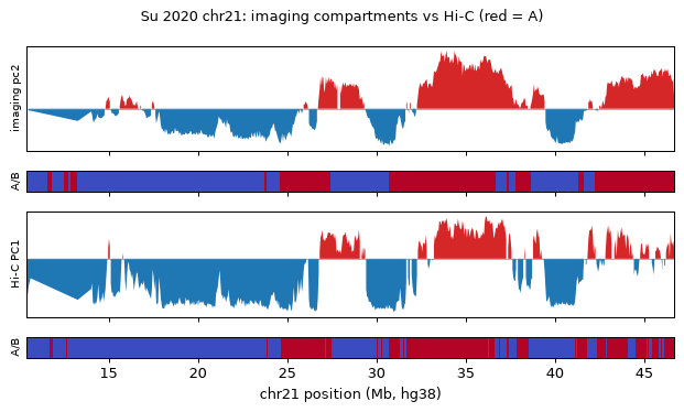
How this compares with the paper. ArcFISH validated this caller on Su 2020 chromosome 2 (250 kb, 3,029 traces), where 84.3 % of the loci share the bulk Hi-C assignment. On chromosome 21 this implementation agrees with the Hi-C compartments at a similar level (the number above), and its track follows Hi-C PC1 closely.
How many traces are needed?
ArcFISH reports that about 30 traces are enough to assign A/B
compartments. trace_ids= restricts the call to a random subset of
chromosome copies; labels are oriented with the gene annotation as above.
rng = np.random.default_rng(0)
copies = su.spots["trace_id"].astype(str).unique()
rows = []
for n in (30, 100, 300):
    for rep in range(2):
        pick = rng.choice(copies, size=n, replace=False)
        c = uc.tl.call_compartments(su, trace_ids=pick, key_added=None).sort_values("start")
        a = c.assign(n_genes=gene_count.loc[c.start].to_numpy()).groupby("cluster").n_genes.mean().idxmax()
        lab = np.where(c.cluster.to_numpy() == a, "A", "B")
        track = c.pc2.to_numpy() * (1 if c.loc[c.cluster == a, "pc2"].mean() > 0 else -1)
        rows.append({"traces": n, "draw": rep, "same label as Hi-C": np.mean(lab == hic_label),
                     "r(pc2, Hi-C PC1)": np.corrcoef(track, pc1)[0, 1]})
pd.DataFrame(rows).round(3)
| traces | draw | same label as Hi-C | r(pc2, Hi-C PC1) | |
|---|---|---|---|---|
| 0 | 30 | 0 | 0.912 | 0.843 |
| 1 | 30 | 1 | 0.865 | 0.827 |
| 2 | 100 | 0 | 0.908 | 0.914 |
| 3 | 100 | 1 | 0.916 | 0.916 |
| 4 | 300 | 0 | 0.911 | 0.921 |
| 5 | 300 | 1 | 0.914 | 0.913 |
Many chromosomes at once (Takei 2021)
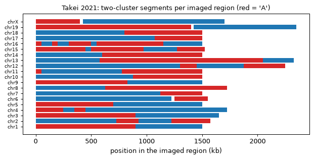
With chrom=None (the default) the caller runs each chromosome and merges
the tables. The Takei 2021 25-kb data have one region of 60 loci per
chromosome (1.5–2.4 Mb) — no longer than a typical compartment, so the two
clusters found inside each region are sub-region structure rather than
genome-wide A/B; the example shows the mechanics and the outputs.
cd = ChromData.from_fofct(CORE)
comps = uc.tl.call_compartments(cd)
seg = cd.intervals["compartments.axes_pc"]
print(f"{len(comps)} loci on {comps.chrom.nunique()} chromosomes -> {len(seg)} segments")

# interval tables map back onto any bin table: label of the overlapping segment per locus
labels = seg.to_bins(cd.bins, how="id", column="label")
print(labels.value_counts().to_dict())
cd.bins.assign(label=labels, pc2=cd.bin_tracks["compartments.axes_pc.pc2"]).head()
1200 loci on 20 chromosomes -> 57 segments
{'B': 676, 'A': 524}
| chrom | start | end | label | pc2 | |
|---|---|---|---|---|---|
| bin_id | |||||
| 0 | chr1 | 135600000 | 135625000 | A | 0.059432 |
| 1 | chr1 | 135625000 | 135650000 | A | 0.049659 |
| 2 | chr1 | 135650000 | 135675000 | A | 0.013774 |
| 3 | chr1 | 135675000 | 135700000 | A | 0.069936 |
| 4 | chr1 | 135700000 | 135725000 | A | 0.073225 |
fig, ax = plt.subplots(figsize=(7, 3.6))
order = sorted(seg.chrom.unique(), key=lambda c: int(c[3:]) if c[3:].isdigit() else 99)
for y, chrom in enumerate(order):
    g = seg[seg.chrom == chrom]
    lo = cd.bins.loc[cd.bins.chrom == chrom, "start"].min()
    ax.broken_barh(list(zip((g.start - lo) / 1e3, (g.end - g.start) / 1e3)), (y - 0.4, 0.8),
                   facecolors=["tab:red" if l == "A" else "tab:blue" for l in g.label])
ax.set_yticks(range(len(order)), order, fontsize=7)
ax.set_xlabel("position in the imaged region (kb)")
ax.set_title("Takei 2021: two-cluster segments per imaged region (red = 'A')", fontsize=10)
plt.tight_layout(); plt.show()
Notes
Name A / B with biology (gene density, active histone marks, Hi-C) through
a_cluster; the default compaction rule is a convention and named the compartments the wrong way round on Su 2020 chr21.n_clusters > 2explores sub-compartments; the labels are then"A"fora_clusterand"B"for every other cluster, so use theclustercolumn.On a backed store the caller reads one chromosome at a time (
get_chrom); it has no streaming mode — the loop and TAD callers do.uchrom.strc.enrichment.add_structural_featuresprojects the stored compartments (label,pc2) onto bins together with TADs and loops (seetad_calling).
Next steps
tad_calling— TADs on the same chr21 loci, imaging vs Hi-C, and the backed / streaming workflow.loop_calling— loops on the Takei 2021 data.