Single-allele domains with FISHnet

TAD callers on tracing data usually pool all traces into one answer per chromosome. FISHnet (Patel et al. 2025, Nature Methods 22:1255, doi:10.1038/s41592-025-02688-1) calls domains on each allele separately, so cell-to-cell variability becomes visible. This tutorial runs uchrom.strc.tad.call_domains_fishnet_trace on one allele and call_domains_fishnet (also uc.tl.call_tads(method="fishnet")) on a sample of alleles, sums them into the ensemble domain mask, and compares the single-allele boundaries with the population boundaries of the ArcFISH caller (call_tads_by_pval). Data: Takei et al. 2021 (Nature 590:344) mESC DNA seqFISH+ at 25 kb, the 60-locus (1.5-Mb) region on chr6 (ds.fetch("takei") downloads the FOF-CT core table 4DNFIHF3JCBY once from 4DN, 22 MB). Runtime: 2–5 minutes (FISHnet runs Louvain many times per allele on the CPU).

How FISHnet works (per allele):

1. Threshold sweep — binarise the allele’s pairwise distance matrix at a series of distance thresholds ((i, j) → 1 if dist ≤ t).

2. Smooth — a (2w)×(2w) boxcar turns the binary map into a weighted graph.

3. Louvain modularity — run Louvain community detection several times per threshold and keep the consensus partition (highest mean adjusted Rand index to the other runs).

4. Plateaus — runs of plateau_size or more consecutive thresholds with the same number of communities; each plateau gives one partition.

5. Clean-up — merge runs shorter than size_exclusion loci and boundaries closer than merge_tol loci.

import time
from pathlib import Path

import numpy as np
import pandas as pd
import matplotlib.pyplot as plt

from chromdata import ChromData
import uchrom as uc
import uchrom.datasets as ds

plt.rcParams["figure.dpi"] = 90

OUT = Path("_out"); OUT.mkdir(exist_ok=True)   # outputs: tutorials/_out/ (ignored by git)
CORE = ds.fetch("takei")                       # Takei 2021 FOF-CT core table (4DN, 22 MB; downloaded once)

Load the traces and pick a chromosome

from uchrom.strc.tad import (FISHnetParams, TADCallerParams, call_domains_fishnet,
                             call_domains_fishnet_trace, call_tads_by_pval)

cd = ChromData.from_fofct(CORE)
CHROM = "chr6"
chrom_bins = cd.bins[cd.bins["chrom"] == CHROM].sort_values("start")
row_of = pd.Series(np.arange(len(chrom_bins)), index=chrom_bins.index)     # bin_id -> matrix row

coverage = (cd.get_chrom(CHROM).spots.groupby("trace_id", observed=True)["bin_id"].nunique()
            / len(chrom_bins))
print(f"{CHROM}: {len(chrom_bins)} loci, {len(coverage)} alleles; "
      f"median coverage {coverage.median():.0%}, {int((coverage >= 0.6).sum())} alleles with ≥ 60 %")

chr6: 60 loci, 415 alleles; median coverage 55%, 179 alleles with ≥ 60 %

One allele

call_domains_fishnet_trace works on one pairwise distance matrix (NaN for undetected loci, which are linearly imputed when impute=True). Build the matrix of the best-covered allele from cd.get_trace and run FISHnet with the paper’s defaults.

def trace_distances(trace_id):
    t = cd.get_trace(trace_id)
    xyz = np.full((len(chrom_bins), 3), np.nan)
    xyz[row_of[t.spots["bin_id"]].to_numpy()] = t.coords          # a locus seen twice keeps its last spot
    return np.linalg.norm(xyz[:, None] - xyz[None], axis=-1)


demo = str(coverage.idxmax())
D = trace_distances(demo)
t0 = time.perf_counter()
res = call_domains_fishnet_trace(D, params=FISHnetParams())      # paper defaults
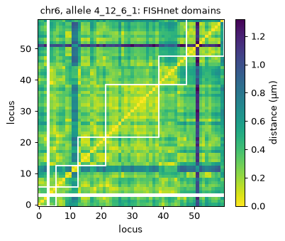
print(f"allele {demo} (coverage {coverage.max():.0%}): {len(res['domains'])} domains from "
      f"{res['n_plateaus']} plateaus, boundaries at loci {res['boundaries']} "
      f"({time.perf_counter() - t0:.1f} s)")

allele 4_12_6_1 (coverage 98%): 6 domains from 5 plateaus, boundaries at loci [6, 13, 22, 39, 48] (33.3 s)

from matplotlib.patches import Rectangle

fig, ax = plt.subplots(figsize=(4.6, 3.8))
im = ax.imshow(D, cmap="viridis_r", origin="lower")
for a, b in res["domains"]:
    ax.add_patch(Rectangle((a - 0.5, a - 0.5), b - a, b - a, fill=False, edgecolor="white", lw=1.5))
ax.set_title(f"{CHROM}, allele {demo}: FISHnet domains", fontsize=10)
ax.set_xlabel("locus"); ax.set_ylabel("locus")
plt.colorbar(im, ax=ax, label="distance (µm)")
plt.tight_layout(); plt.show()

Many alleles → ensemble domain mask

call_domains_fishnet runs every selected allele of a chromosome. We pick 40 random alleles with at least 60 % of the loci detected (trace_ids=) and lighten the sweep (10 Louvain runs at each of 30 thresholds, plateaus of 3) to keep the runtime down. The per-allele domains are stored as a domain interval table under "tads.fishnet"; the ensemble domain mask — for each locus pair, how often (alleles × plateaus) both loci share a domain — under "tads.fishnet.ensemble".

rng = np.random.default_rng(0)
eligible = coverage[coverage >= 0.6].index.astype(str)
sample = rng.choice(eligible, size=40, replace=False)
FAST = FISHnetParams(n_louvain_runs=10, max_thresholds=30, plateau_size=3)

t0 = time.perf_counter()
fn = call_domains_fishnet(cd, chrom=CHROM, trace_ids=sample, params=FAST)
n_called = fn.trace_id.nunique()
print(f"{len(fn)} domains on {n_called} of {len(sample)} alleles ({time.perf_counter() - t0:.0f} s)")
print(cd.intervals)
fn.head()

202 domains on 40 of 40 alleles (124 s)
IntervalStore({'tads.fishnet': <domain, 202 rows>})

	chrom	trace_id	domain_idx	start	end	start_bin	end_bin
0	chr6	0_7_6_0	0	49375000	49575000	0	7
1	chr6	0_7_6_0	1	49575000	49850000	7	18
2	chr6	0_7_6_0	2	49850000	50025000	18	25
3	chr6	0_7_6_0	3	50025000	50175000	25	31
4	chr6	0_7_6_0	4	50175000	50375000	31	39

from uchrom.fea import distance_map

ens = cd.results["tads.fishnet.ensemble"][CHROM]       # one entry per chromosome
dm = distance_map(cd, CHROM)                            # all alleles, median

fig, axes = plt.subplots(1, 2, figsize=(7, 3.1))
im0 = axes[0].imshow(dm.matrix, cmap="viridis_r", origin="lower")
axes[0].set_title(f"median distance ({dm.n_traces} alleles)", fontsize=10)
plt.colorbar(im0, ax=axes[0], label="µm")
im1 = axes[1].imshow(ens["mask"], cmap="magma", origin="lower")
axes[1].set_title(f"FISHnet ensemble mask ({ens['n_traces']} alleles)", fontsize=10)
plt.colorbar(im1, ax=axes[1], label="alleles × plateaus")
for ax in axes:
    ax.set_xlabel("locus")
plt.tight_layout(); plt.show()

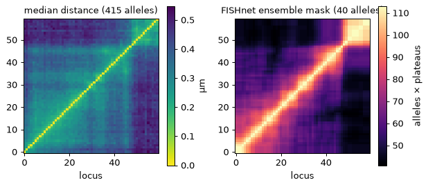
The block structure of the ensemble mask follows the low-distance blocks of the population map: the population pattern is the sum of domains that individual alleles form, each at somewhat different places.

Cell-to-cell variability

per_allele = fn.groupby("trace_id", observed=True).size()
size_kb = (fn.end - fn.start) / 1e3
fig, axes = plt.subplots(1, 2, figsize=(7, 2.8))
axes[0].hist(per_allele, bins=np.arange(per_allele.max() + 2) - 0.5, color="tab:blue", edgecolor="k")
axes[0].set_xlabel("domains per allele"); axes[0].set_ylabel("alleles")
axes[1].hist(size_kb, bins=20, color="tab:green", edgecolor="k")
axes[1].set_xlabel("domain size (kb)"); axes[1].set_ylabel("domains")
plt.tight_layout(); plt.show()
print(f"domains per allele: median {per_allele.median():.0f} (range {per_allele.min()}–{per_allele.max()}); "
      f"domain size: median {size_kb.median():.0f} kb")

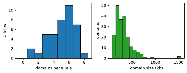
domains per allele: median 5 (range 1–8); domain size: median 275 kb

Single-allele boundaries vs population boundaries

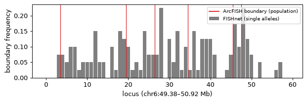
The ArcFISH preprint finds that population boundaries with larger test statistics occur more often in single cells (Pearson r = 0.45 with FISHnet on these data). A simple version of that check: how often is each locus a FISHnet boundary across the alleles, and is that frequency higher at the boundaries the population caller (ArcFISH window ±100 kb) finds?

starts = ens["bin_ids"][:, 0]
freq = np.bincount(fn.loc[fn.start_bin > 0, "start_bin"], minlength=len(starts)) / n_called

pop = call_tads_by_pval(cd, chrom=CHROM, params=TADCallerParams(window_bp=2e5, hierarchical=False),
                        key_added=None)
pop_idx = np.searchsorted(starts, pop.start.iloc[1:].to_numpy())
near = np.zeros(len(starts), bool)
for k in pop_idx:
    near[max(k - 1, 0):k + 2] = True                    # boundary locus ± 1
print(f"{len(pop_idx)} population boundaries; FISHnet boundary frequency "
      f"{freq[near].mean():.3f} within ±1 locus of them vs {freq[~near].mean():.3f} elsewhere "
      f"({freq[near].mean() / freq[~near].mean():.1f}×)")

fig, ax = plt.subplots(figsize=(7, 2.4))
ax.bar(np.arange(len(starts)), freq, color="tab:grey", width=0.9, label="FISHnet (single alleles)")
for k in pop_idx:
    ax.axvline(k - 0.5, color="tab:red", lw=1)
ax.plot([], [], color="tab:red", label="ArcFISH boundary (population)")
ax.set_xlabel(f"locus ({CHROM}:{starts[0] / 1e6:.2f}–{chrom_bins.end.max() / 1e6:.2f} Mb)")
ax.set_ylabel("boundary frequency"); ax.legend(fontsize=8, loc="upper right")
plt.tight_layout(); plt.show()

6 population boundaries; FISHnet boundary frequency 0.106 within ±1 locus of them vs 0.052 elsewhere (2.0×)

Notes: which caller when

• FISHnet (this tutorial) — per-allele domains; questions such as which alleles fold alike? or how variable are boundaries?

• ArcFISH p-value caller (tad_calling) — population boundaries with FDR control and a hierarchy.

• Directionality index (call_tads_di, tad_calling) — Hi-C contact matrices.

Parameter	Effect
plateau_size	larger → fewer, more stable partitions (paper: 4)
window_size	boxcar half-width in loci (paper: 2)
max_thresholds / threshold_step	density of the sweep; runtime grows linearly
n_louvain_runs	stability of the consensus (paper: 20); runtime grows linearly
min_coverage	skip alleles with fewer detected loci (default 60 %)
impute	interpolate undetected loci before thresholding

The upstream implementation (github.com/RohanpatelUpenn/FISHnet, no open-source licence) uses its own Louvain solver; this independent re-implementation uses networkx.algorithms.community.louvain_communities, so it is slow: several seconds per allele with the light settings above. Alleles are independent — split trace_ids across processes for whole data sets.

Next steps

• tad_calling — population TADs, hierarchy, streaming on backed stores.

• loop_calling — loops on the same data.