Contact-map cell embedding with FastHigashi¶

FastHigashi (Zhang et al. 2022, Cell Systems) embeds single-cell Hi-C maps by a tensor decomposition of all cells’ contact maps, chromosome by chromosome. This tutorial runs it on sci-Hi-C of two human cell lines. It covers the whole path:

write the Higashi input files with uchrom.io.contacts (make_higashi_config, write_label_info);
run FastHigashi through uchrom.emb.higashi.run, which stores the embedding in cd.cellm["higashi"];
score the embedding against the known cell types (ARI / NMI);
compute t-SNE / UMAP and Leiden clusters with uchrom.emb.embed_cells / cluster_cells.
Data: Kim et al. 2020 (Nat. Commun. 11:6386) sci-Hi-C of an H1 ES cell (H1Esc) and foreskin fibroblast (HFF) mix: 1,931 cells at 500 kb, hg19, with cell-type labels. ds.fetch("kim2020_scihic") downloads the contact matrices (H1Esc-HFF.R1.tar.gz, 128 MB) and the labels (H1Esc-HFF.R1.labeled) once from the Noble lab; the tarball is extracted next to them on first run.
Runtime: 3–5 min on a laptop CPU (FastHigashi itself takes 2–4 min), for 150 cells of each type picked at random.
Requirements: FastHigashi is an optional dependency and is not on PyPI. Install it from GitHub in an environment with NumPy < 2, because FastHigashi 0.1.1a0 calls np.array(..., copy=False):
```
pip install "numpy<2" opt_einsum tqdm psutil
pip install git+https://github.com/ma-compbio/Fast-Higashi
```

import importlib.util
import json
import shutil
import tarfile
import time
import warnings
from pathlib import Path

import matplotlib.pyplot as plt
import numpy as np
import pandas as pd
from sklearn.cluster import KMeans
from sklearn.metrics import adjusted_rand_score, normalized_mutual_info_score

from chromdata import ChromData
import uchrom.datasets as ds
from uchrom import emb
from uchrom.emb.higashi import run as higashi_run
from uchrom.io.contacts import make_higashi_config, write_label_info

plt.rcParams["figure.dpi"] = 90
warnings.filterwarnings("ignore", message="IProgress not found")   # tqdm, imported by umap-learn

OUT = Path("_out"); OUT.mkdir(exist_ok=True)   # outputs: tutorials/_out/ (ignored by git)
if importlib.util.find_spec("fasthigashi") is None:
    raise ImportError("FastHigashi is not installed: see the install commands in the first cell")
print("numpy", np.__version__)
T0 = time.time()

numpy 1.26.4

1. The data¶

Each cell’s .matrix file is a sparse list bin1, bin2, count, weight, chrom1, chrom2. bin1 and bin2 are genome-wide 500 kb bin numbers: the bins of chr1, then chr2, and so on, in hg19 order. ds.fetch returns the folder with the tarball and the labels; the tarball is extracted there once.

KIM2020 = ds.fetch("kim2020_scihic")                 # folder: H1Esc-HFF.R1.tar.gz + H1Esc-HFF.R1.labeled
matrices_dir, labels_path = KIM2020 / "H1Esc-HFF.R1", KIM2020 / "H1Esc-HFF.R1.labeled"
if not matrices_dir.exists():                        # one .matrix file per cell
    with tarfile.open(KIM2020 / "H1Esc-HFF.R1.tar.gz", "r:gz") as tf:
        tf.extractall(KIM2020, filter="data")

labels = pd.read_csv(labels_path, sep="\t", header=None, names=["matrix", "cell_type"])
print(f"{len(labels):,} cells:", labels["cell_type"].value_counts().to_dict())
pd.read_csv(matrices_dir / labels["matrix"].iloc[0], sep="\t", header=None, nrows=3,
            names=["bin1", "bin2", "count", "weight", "chrom1", "chrom2"])

1,931 cells: {'HFF': 1181, 'H1Esc': 750}

	bin1	bin2	count	weight	chrom1	chrom2
0	1868	1868	1	0.250000	human_chr5	human_chr5
1	588	3317	1	0.288675	human_chr2	human_chr9
2	1774	4583	1	0.218218	human_chr5	human_chr14

2. Pick the cells and convert their contacts to Higashi input¶

We pick 150 H1Esc and 150 HFF cells at random (seed 0). FastHigashi needs population diversity, and more cells give a better embedding but take longer.

Each chromosome’s first genome-wide bin follows from the hg19 chromosome sizes: it is the number of 500 kb bins of all chromosomes before it. Do not take the smallest bin seen in the data instead. On the acrocentric chromosomes (13, 14, 15, 21, 22) the unmappable short arm has no contacts, so that would shift every contact by up to 19 Mb. The check below makes sure that every observed bin falls inside its chromosome.

RESOLUTION = 500_000
HG19 = {"chr1": 249250621, "chr2": 243199373, "chr3": 198022430, "chr4": 191154276, "chr5": 180915260,
        "chr6": 171115067, "chr7": 159138663, "chr8": 146364022, "chr9": 141213431, "chr10": 135534747,
        "chr11": 135006516, "chr12": 133851895, "chr13": 115169878, "chr14": 107349540, "chr15": 102531392,
        "chr16": 90354753, "chr17": 81195210, "chr18": 78077248, "chr19": 59128983, "chr20": 63025520,
        "chr21": 48129895, "chr22": 51304566, "chrX": 155270560}           # chrY has no contacts here
n_bins = {c: -(-size // RESOLUTION) for c, size in HG19.items()}
offset = dict(zip(n_bins, np.r_[0, np.cumsum(list(n_bins.values()))[:-1]]))

N_PER_TYPE = 150
sub = pd.concat([labels[labels["cell_type"] == t].sample(N_PER_TYPE, random_state=0)
                 for t in ("H1Esc", "HFF")]).reset_index(drop=True)
sub["cell_name"] = sub["matrix"].str.removesuffix("_500000.matrix")


def matrix_to_higashi(path):
    m = pd.read_csv(path, sep="\t", header=None, names=["bin1", "bin2", "count", "weight", "chrom1", "chrom2"])
    c1, c2 = m["chrom1"].str.removeprefix("human_"), m["chrom2"].str.removeprefix("human_")
    b1, b2 = m["bin1"] - c1.map(offset), m["bin2"] - c2.map(offset)
    assert ((b1 >= 0) & (b1 < c1.map(n_bins)) & (b2 >= 0) & (b2 < c2.map(n_bins))).all(), path.name
    return pd.DataFrame({"chrom1": c1, "pos1": b1 * RESOLUTION, "chrom2": c2, "pos2": b2 * RESOLUTION,
                         "count": m["count"]})


work = OUT / "higashi_kim2020"
shutil.rmtree(work, ignore_errors=True)           # FastHigashi caches per input set: start clean
higashi_dir = work / "input"
(higashi_dir / "data").mkdir(parents=True, exist_ok=True)
files, n_contacts = [], []
for row in sub.itertuples():
    contacts = matrix_to_higashi(matrices_dir / row.matrix)
    path = higashi_dir / "data" / f"{row.cell_name}.txt"
    contacts.to_csv(path, sep="\t", index=False, header=False)      # chrom1 pos1 chrom2 pos2 count
    files.append(str(path.resolve()))
    n_contacts.append(int(contacts["count"].sum()))
sub["n_contacts"] = n_contacts
print(f"{len(sub)} cells; median contacts per cell:", sub.groupby("cell_type")["n_contacts"].median().to_dict())

300 cells; median contacts per cell: {'H1Esc': 7570.0, 'HFF': 2794.0}

The remaining input files are the following:

filelist.txt: one contact file per cell.
label_info.pickle: per-cell metadata, in the same order. FastHigashi returns the embedding in this order.
chromsizes.tsv
config.JSON: genome, resolution, chromosomes and paths.

write_higashi_inputs writes all of them for .pairs files. Here the contacts come from .matrix files, so we call its helpers write_label_info and make_higashi_config directly.

(higashi_dir / "filelist.txt").write_text("\n".join(files) + "\n")
write_label_info(sub[["cell_name", "cell_type", "n_contacts"]], higashi_dir / "label_info.pickle")
pd.Series(HG19).to_csv(higashi_dir / "chromsizes.tsv", sep="\t", header=False)
config = make_higashi_config(data_dir=str(higashi_dir), genome_reference="hg19", resolution=RESOLUTION,
                             chrom_list=list(HG19),
                             overrides={"genome_reference_path": str(higashi_dir / "chromsizes.tsv")})
(higashi_dir / "config.JSON").write_text(json.dumps(config, indent=2))
print(sorted(p.name for p in higashi_dir.iterdir()))
{k: config[k] for k in ("resolution", "input_format", "contact_header", "header_included")}

['chromsizes.tsv', 'config.JSON', 'data', 'filelist.txt', 'label_info.pickle']

{'resolution': 500000,
 'input_format': 'higashi_v2',
 'contact_header': ['chrom1', 'pos1', 'chrom2', 'pos2', 'count'],
 'header_included': False}

3. A `ChromData` of the cells¶

These data have contacts but no 3-D coordinates, so the ChromData has cells and no spots. This is the same layout as the scHiCAR store in cell_embeddings.ipynb. higashi.run matches the rows of the embedding to cd.cells by the cell_name column.

no_spots = pd.DataFrame({c: pd.Series(dtype=t) for c, t in
                         [("chrom", str), ("start", np.int64), ("end", np.int64), ("trace_id", str), ("cell_id", str)]})
cd = ChromData(np.zeros((0, 3)), no_spots,
               cells=sub.set_index(pd.Index(sub["cell_name"], name="cell_id"))[["cell_name", "cell_type", "n_contacts"]],
               uns={"genome_assembly": "hg19", "source": "Kim et al. 2020 sci-Hi-C (H1Esc-HFF.R1), 500 kb"})
print(cd.n_cells, "cells;", list(cd.cells.columns))

300 cells; ['cell_name', 'cell_type', 'n_contacts']

4. Run FastHigashi¶

higashi.run drives FastHigashi’s four steps (fast_process_data, prep_dataset, run_model, fetch_cell_embedding). It writes the chosen embedding variant to cd.cellm["higashi"], with rows in the order of cd.cells. It also makes pin_memory a no-op on machines without CUDA, such as Apple Silicon.

We pass the following options:

do_conv, do_rwr, do_col: smoothing, random walk with restart and column normalisation of the very sparse maps;
rank 64;
embed_variant="embed_l2_norm_correct_coverage_fh": the embedding after FastHigashi regresses out each cell’s coverage. The HFF cells here have about 3× fewer contacts than the H1Esc cells, so coverage alone would separate the two types in the uncorrected embedding.

wrapper_factory lets us keep the FastHigashi object, so that we can compare the variants afterwards. FastHigashi prints a lot of progress output, so we send it to a log file. Its initialisation is random, so we seed NumPy and PyTorch.

import contextlib
import os
import sys


@contextlib.contextmanager
def to_log(path):
    # route Python-level and subprocess output (fd 1 / 2) to a file
    sys.stdout.flush(); sys.stderr.flush()
    with open(path, "w") as log, contextlib.redirect_stdout(log), contextlib.redirect_stderr(log):
        saved = os.dup(1), os.dup(2)
        os.dup2(log.fileno(), 1); os.dup2(log.fileno(), 2)
        try:
            yield
        finally:
            log.flush()
            os.dup2(saved[0], 1); os.dup2(saved[1], 2)
            os.close(saved[0]); os.close(saved[1])


models = []


def keep_model(*args):
    from fasthigashi.FastHigashi_Wrapper import FastHigashi
    models.append(FastHigashi(*args))
    return models[-1]


import torch

torch.manual_seed(0); np.random.seed(0)          # FastHigashi's initialisation and final SVD are random
log_path = work / "fasthigashi.log"
t = time.time()
with to_log(log_path):
    cd = higashi_run(cd, contacts_dir=higashi_dir, rank=64, cache_dir=work / "cache", result_dir=work / "result",
                     wrapper_kwargs={"do_conv": True, "do_rwr": True, "do_col": True},
                     embed_variant="embed_l2_norm_correct_coverage_fh", wrapper_factory=keep_model)
print(f"FastHigashi: {time.time() - t:.0f} s; cd.cellm['higashi'] {cd.cellm['higashi'].shape}; "
      f"log in {log_path}")
print(*[line for line in log_path.read_text().splitlines() if "pass qc" in line or line.startswith("PARAFAC2")][-3:],
      sep="\n")
{k: v for k, v in cd.uns["higashi"].items() if k not in ("config_path", "result_dir")}

FastHigashi: 178 s; cd.cellm['higashi'] (300, 64); log in _out/higashi_kim2020/fasthigashi.log
PARAFAC2 re=0.613 1.10e-02 variation min4.3e-03 at chrom 22, max1.9e-02 at chrom 17 takes 8.6s
PARAFAC2 re=0.611 5.91e-03 variation min1.7e-03 at chrom 22, max1.1e-02 at chrom 17 takes 9.3s
PARAFAC2 re=0.610 3.69e-03 variation min8.8e-04 at chrom 22, max6.8e-03 at chrom 17 takes 8.9s

{'method': 'fast',
 'rank': 64,
 'embed_variant': 'embed_l2_norm_correct_coverage_fh'}

5. Score the embedding against the cell types¶

We cluster the embedding into k = 2 groups with k-means and compare the groups with the labels by ARI and NMI (0 = chance, 1 = perfect).

FastHigashi also flags cells by quality. A cell passes when enough bins of every chromosome have contacts; the flag is written to qc.npy in the cache directory. We score all cells and the cells that pass separately. The table also lists the other embedding variants that FastHigashi returned.

y = cd.cells["cell_type"].to_numpy()
qc = np.load(work / "cache" / "qc.npy") > 0             # in label_info order = cd.cells order
cd.cells["fasthigashi_qc"] = pd.Categorical(np.where(qc, "pass", "fail"))
print("cells passing FastHigashi's QC:", pd.crosstab(cd.cells["cell_type"], qc).rename(columns={True: "pass", False: "fail"}).to_dict("index"))


def score(x):
    pred = KMeans(2, n_init=10, random_state=0).fit_predict(x)
    pred_qc = KMeans(2, n_init=10, random_state=0).fit_predict(x[qc])
    return {"ARI (all)": adjusted_rand_score(y, pred), "NMI (all)": normalized_mutual_info_score(y, pred),
            "ARI (QC pass)": adjusted_rand_score(y[qc], pred_qc),
            "|r| dim 1 vs log contacts": abs(np.corrcoef(x[:, 0], np.log(cd.cells["n_contacts"]))[0, 1])}


variants = models[0].embedding_storage                   # every variant FastHigashi computed
table = pd.DataFrame({k: score(np.asarray(v)) for k, v in variants.items()
                      if k.startswith("embed_") and k != "embed_all"}).T.round(3)
table.index.name = "variant"
print("stored in cd.cellm['higashi']:", cd.uns["higashi"]["embed_variant"])
table

cells passing FastHigashi's QC: {'H1Esc': {'fail': 60, 'pass': 90}, 'HFF': {'fail': 118, 'pass': 32}}

stored in cd.cellm['higashi']: embed_l2_norm_correct_coverage_fh

	ARI (all)	NMI (all)	ARI (QC pass)	\|r\| dim 1 vs log contacts
variant
embed_raw	0.052	0.048	1.0	0.629
embed_l2_norm	0.209	0.201	1.0	0.757
embed_correct_coverage_fh	0.003	0.008	1.0	0.040
embed_l2_norm_correct_coverage_fh	0.452	0.388	1.0	0.291

On the cells that pass QC, k-means on any variant splits H1Esc from HFF perfectly (ARI 1). The cells that fail are mostly HFF cells with few contacts. For them, coverage dominates the uncorrected variants, and the ARI over all cells drops. The stored variant regresses out coverage and then L2-normalises (embed_l2_norm_correct_coverage_fh). It roughly doubles the all-cell ARI of embed_l2_norm, but does not remove the effect; the unnormalised corrected variant is unstable between runs. More cells, or a minimum number of contacts per cell, help as well. The all-cell numbers also depend on the random initialisation: without seeds, the ARI of the stored variant ranged from 0.42 to 0.51 in our runs, while the QC-pass ARI stayed at 1.

6. t-SNE / UMAP and Leiden clusters with `uchrom.emb`¶

The FastHigashi embedding is a cells × 64 matrix, so it can go through embed_cells like any other features. source="higashi" is shown as the Hi-C modality, and normalization="none" uses the values as they are. This gives higashi_pca, higashi_tsne and higashi_umap, recorded in cd.uns["embeddings"] for the web browser. cluster_cells then computes Leiden clusters.

emb.embed_cells(cd, source="higashi", matrix=cd.cellm["higashi"], normalization="none", n_pcs=20,
                features="FastHigashi (rank 64, conv + rwr + col), coverage-corrected, L2-normalised")
leiden = emb.cluster_cells(cd, use="higashi_pca", resolution=0.5, key_added="leiden_higashi")
print(f"{leiden.nunique()} Leiden clusters: ARI {adjusted_rand_score(y, leiden):.3f}, "
      f"NMI {normalized_mutual_info_score(y, leiden):.3f}")
display(pd.crosstab(leiden, [cd.cells["cell_type"], cd.cells["fasthigashi_qc"]]).rename_axis(index="leiden_higashi"))

xy = cd.cellm["higashi_umap"]
fig, axes = plt.subplots(1, 2, figsize=(7, 3.2))
for t, color in [("H1Esc", "tab:red"), ("HFF", "tab:blue")]:
    m = y == t
    axes[0].scatter(xy[m, 0], xy[m, 1], s=8, lw=0, color=color, label=t)
axes[0].legend(fontsize=8, frameon=False); axes[0].set_title("cell type", fontsize=9)
sc = axes[1].scatter(xy[:, 0], xy[:, 1], s=8, lw=0, c=np.log10(cd.cells["n_contacts"]), cmap="viridis")
fig.colorbar(sc, ax=axes[1], label="log10 contacts"); axes[1].set_title("coverage", fontsize=9)
for ax in axes:
    ax.set_xticks([]); ax.set_yticks([]); ax.set_xlabel("UMAP 1", fontsize=8); ax.set_ylabel("UMAP 2", fontsize=8)
fig.suptitle("FastHigashi embedding, UMAP (embed_cells)", fontsize=9)
fig.tight_layout()

3 Leiden clusters: ARI 0.197, NMI 0.312

cell_type	H1Esc		HFF
fasthigashi_qc	fail	pass	fail	pass
leiden_higashi
0	52	22	117	11
1	8	68	1	0
2	0	0	0	21

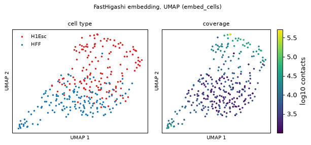
../_images/1481f68325eeba0c89cfd728308a7cd0a00f68c3d0f6f3af2d7f6c7a4cb96dd0.png

Leiden gives the same picture as k-means. Most cells that pass QC fall into two clusters, one for each cell type, while most low-coverage cells form a third, mixed cluster. The UMAP shows this too: the cells with many contacts separate by type, and those with few contacts mix.

7. Store the result¶

The embedding and its provenance stay with the cells: cd.cellm["higashi"] holds the embedding, and cd.uns["higashi"] holds the method, rank, variant and FastHigashi’s config and result directory. FastHigashi’s imputed per-cell maps can be large, so they stay in that result directory; ChromData keeps no per-cell pairwise matrices.

path = OUT / "kim2020_higashi.chromdata.zarr"
cd.write(path)
back = ChromData.read(path)
print(path, "| cellm:", sorted(back.cellm),
      "| equal:", np.allclose(back.cellm["higashi"], cd.cellm["higashi"]))
print("result directory:", back.uns["higashi"]["result_dir"])
print(f"total runtime {time.time() - T0:.0f} s")

_out/kim2020_higashi.chromdata.zarr | cellm: ['higashi', 'higashi_pca', 'higashi_tsne', 'higashi_umap'] | equal: True
result directory: _out/higashi_kim2020/result
total runtime 193 s

Next steps¶

cell_embeddings.ipynb: RNA, ATAC, contact-map (scHiCluster) and IF embeddings of the same cells, Leiden clusters, marker features, and how the web browser reads cd.uns["embeddings"].
chromdata_basics.ipynb: the ChromData container.
To embed all 1,931 cells, use sub = labels.copy() instead of the random sample. This takes longer on a CPU; FastHigashi uses a CUDA GPU when one is available.