Spatial variation of 3-D genome features across a tissue

Spatial Hi-C-RNA (Guo et al. 2026, Cell) measures contacts and the transcriptome in the same 20-µm spots of a coronal mouse-brain section. This tutorial asks of each spot’s global 3-D genome features — the share of short- and long-range contacts, the decay of contacts with distance, the cis fraction — whether they vary across the tissue, and whether they vary beyond what the spots’ transcriptomes say:

1. per-spot features from the contact-distance histograms stored in the atlas store (uchrom.fea.contact_features);

2. the tissue: maps, anatomical regions from marker genes, the paper’s short / long-range pattern;

3. the barcode stripes of the microfluidic array and their removal (uchrom.spatial.destripe);

4. spatial tests — Moran’s I and SPARK-X — raw and adjusted for depth and for the spot’s RNA (uchrom.spatial).

Data: atlas store hicrna_mouse_brain (Guo et al. 2026, GEO GSE311199; 2 sections, 12,474 spots), opened over HTTP — only the cells table, the positions and the per-spot histograms are read. The histograms come from one pass over the published pairs (apps/atlas/recipes/spatial_hicrna/slurm/contact_stats.sbatch). Runtime: a few minutes.

import time

import matplotlib.pyplot as plt
import numpy as np
import pandas as pd
from scipy import stats

import uchrom.datasets as ds
from uchrom.fea import ContactFeatureParams, contact_features
from uchrom.pl import plot_spatial
from uchrom.spatial import destripe, smooth_share, sparkx, spatial_autocorr, spatial_neighbors

plt.rcParams["figure.dpi"] = 90
cd = ds.load("hicrna_mouse_brain")
print(cd)
print({k: v.shape for k, v in cd.cellm.items() if k.startswith("contacts")})
print(cd.uns["contact_stats"]["contacts"]["source"])

ChromData (backed: hicrna_mouse_brain.chromdata.zarr): n_spots=0, n_traces=0, n_cells=12474, n_bins=5462
  spots:   ['chrom', 'start', 'end', 'trace_id', 'cell_id', 'bin_id']
  cells:   ['section', 'barcode', 'array_row', 'array_col', 'grid_col', 'grid_row', 'image_x', 'image_y', 'rna_umi', 'rna_genes', 'hic_contacts', 'hic_cis_fraction', 'in_published_analysis', 'cell_type', 'cell_type_confidence', 'cluster_cellcharter', 'cluster_cellcharter_fh', 'cluster_cellcharter_concat', 'rna.Ttr', 'rna.Sec14l4', 'rna.Igf2', 'rna.Ermn', 'rna.Apod', 'rna.Cnp', 'rna.Gfap', 'rna.Mal', 'rna.Cldn11', 'rna.Ptgds', 'rna.Mag', 'rna.Htr2c', 'rna.Gpr88', 'rna.Pdlim2', 'rna.Hba-a1', 'rna.Plekhb1', 'rna.Npy', 'rna.Penk', 'rna.Cryab', 'rna.Ndnf', 'rna.Car2', 'rna.Hmgb2', 'rna.Mt1', 'rna.Mog', 'rna.Gjb1', 'rna.Gjc3', 'rna.Gpr37', 'rna.Ugt8a', 'rna.Bcas1', 'rna.Gjc2', 'rna.Tmem88b', 'rna.Mt2', 'rna.Gsn', 'rna.Olig1', 'rna.Zfp503', 'rna.Aspa', 'rna.Csrp1', 'rna.Lpar1', 'rna.Tmem63a', 'rna.Cnr1', 'rna.Olig2', 'rna.Kl', 'rna.Dio2', 'rna.Hbb-bs', 'rna.Sult1a1', 'rna.Ctgf', 'rna.Opalin', 'rna.Ppp1r14a', 'rna.Rgs9', 'rna.Prr5l', 'rna.Sowaha', 'rna.Ezr', 'rna.Dbi', 'rna.Unc93b1', 'rna.Plekhh1', 'rna.S100a1', 'rna.Aqp4', 'rna.Sepp1', 'rna.Daam2', 'rna.Sept4', 'rna.mt-Tl1', 'rna.Nkx6-2', 'rna.Cers2', 'rna.Cd63', 'rna.Tst', 'rna.Vim', 'rna.Laptm5', 'rna.Serpinb1a', 'rna.Phlda3', 'rna.Zcchc24', 'rna.Slco1c1', 'rna.Rps8', 'rna.Efnb3', 'rna.Sst', 'rna.Vtn', 'rna.Lzts2', 'rna.Rpl18a', 'rna.Prdx6', 'rna.Elovl1', 'rna.Sdc4', 'rna.Pde8a', 'rna.Pllp', 'rna.Rassf2', 'rna.Hba-a2', 'rna.Pla2g16', 'rna.C1qc', 'rna.Ppp1r1b', 'rna.Rplp1', 'rna.Gja1', 'rna.S1pr1', 'rna.Siglech', 'rna.Scube1', 'rna.Adgrf5', 'rna.Cmtm5', 'rna.Thrsp', 'rna.Padi2', 'rna.Fam107a', 'rna.S100b', 'rna.Sall1', 'rna.Pcbp4', 'rna.Snap25', 'rna.Rbfox3', 'rna.Slc17a7', 'rna.Slc17a6', 'rna.Gad1', 'rna.Gad2', 'rna.Slc32a1', 'rna.Pvalb', 'rna.Vip', 'rna.Lamp5', 'rna.Cux2', 'rna.Rorb', 'rna.Fezf2', 'rna.Bcl11b', 'rna.Tbr1', 'rna.Satb2', 'rna.Mbp', 'rna.Plp1', 'rna.Pdgfra', 'rna.Aldh1l1', 'rna.Slc1a3', 'rna.Cx3cr1', 'rna.P2ry12', 'rna.Csf1r', 'rna.Pecam1', 'rna.Cldn5', 'rna.Flt1', 'rna.Dcn', 'rna.Reln', 'rna.Calb1', 'rna.Calb2', 'rna.Prox1', 'rna.Neurod6', 'rna.Camk2a', 'rna.Nrgn', 'centroid_x', 'centroid_y', 'image_centroid_x', 'image_centroid_y', 'contacts.n_cis', 'contacts.n_trans'] (12474 cells)
  cellm:   {'rna_pca': (12474, 30), 'rna_umap': (12474, 2), 'published_scvi_umap': (12474, 2), 'published_xfh_umap': (12474, 2), 'published_xconcat_umap': (12474, 2), 'contacts.distance': (12474, 132), 'contacts.cis': (12474, 21), 'contacts.trans': (12474, 21), 'contacts.orientation': (12474, 4, 132)}
  uns:     ['genome_assembly', 'source', 'title', 'doi', 'geo', 'coordinate_status', 'spot_mask', 'cell_spatial', 'linked_images', 'linked_anndata', 'embeddings', 'linked_scool', 'linked_cool', 'contacts_stats', 'linked_bin_matrices', 'ssab_layout_check', 'contact_stats']
  linked_adata: lazy
{'contacts.distance': (12474, 132), 'contacts.cis': (12474, 21), 'contacts.trans': (12474, 21), 'contacts.orientation': (12474, 4, 132)}
GSE311199 .nodups.pairs.gz, apps/atlas/recipes/spatial_hicrna/slurm/spatial_pairs_stats.py (MAPQ >= 30, in-tissue spots, main chromosomes)

1. Global features of every spot

contact_features reads cellm["contacts.distance"] — per spot the cis contacts in log2 distance bins from 2.5 kb (8 per octave, the bins of scHiCluster) — and contacts.cis / contacts.trans. With ContactFeatureParams.guo2026() the short / long-range ratio is the paper’s: contacts under 5 kb left out, short = 207 kb – 1.97 Mb, long = 18.8 – 53.1 Mb. The features are written to cd.cells as contacts.*.

t = time.time()
f = contact_features(cd, params=ContactFeatureParams.guo2026())
print(f"{len(f):,} spots in {time.time() - t:.1f} s")
f[["n_cis", "cis_fraction", "frac_short", "frac_long", "short_long_ratio", "frac_2M_12M",
   "ps_slope_100k_1M", "ps_slope_1M_10M"]].describe().round(3)

12,474 spots in 0.5 s

	n_cis	cis_fraction	frac_short	frac_long	short_long_ratio	frac_2M_12M	ps_slope_100k_1M	ps_slope_1M_10M
count	1.247400e+04	12474.000	12474.000	12474.000	12474.000	12474.000	12474.000	12474.000
mean	5.846989e+05	0.937	0.280	0.098	2.916	0.131	-0.987	-1.301
std	7.931067e+05	0.005	0.013	0.011	0.450	0.008	0.022	0.080
min	3.320000e+02	0.913	0.176	0.035	1.517	0.053	-1.317	-1.521
25%	2.475610e+05	0.934	0.271	0.090	2.583	0.126	-0.998	-1.359
50%	4.338200e+05	0.938	0.281	0.097	2.892	0.131	-0.987	-1.305
75%	6.807200e+05	0.941	0.289	0.105	3.216	0.136	-0.975	-1.246
max	3.302210e+07	0.964	0.379	0.155	9.333	0.193	-0.495	-0.406

The barcode channels at the edge of the array carry several times the median contacts — the first and last rows, and the last column (3.6–10×) — one column of section r2 is nearly empty (a dead channel), and some spots are shallow. Kept: spots with at least 50,000 contacts, off the edge rows, the dead columns and any row or column whose median exceeds 2.5× the section’s.

c = cd.cells.copy()
c.index = [str(i) for i in cd._cell_ids_axis()]
c = c.join(f)
c["log_contacts"] = np.log10(c["hic_contacts"])
qc = np.zeros(len(c), bool)
for sec, g in c.groupby("section", observed=True):
    i = c.index.get_indexer(g.index)
    y, x, n = g.centroid_y.to_numpy(), g.centroid_x.to_numpy(), g.hic_contacts.to_numpy()
    med, col_median, row_median = np.median(n), pd.Series(n).groupby(x).median(), pd.Series(n).groupby(y).median()
    dead = np.isin(x, col_median.index[col_median < 0.05 * med])
    hot = np.isin(x, col_median.index[col_median > 2.5 * med]) | np.isin(y, row_median.index[row_median > 2.5 * med])
    qc[i] = (n >= 50_000) & (y != y.min()) & (y != y.max()) & ~dead & ~hot
c["qc"] = qc
print(c.groupby("section", observed=True)["qc"].agg(["sum", "size"]))

                 sum  size
section                   
mouse_brain_r1  6050  6275
mouse_brain_r2  5766  6199

2. The tissue

The short / long-range ratio next to two marker genes (log1p CP10k of the spot’s RNA): white matter (Mbp) and the dentate gyrus (Prox1).

q = c[c.qc]
fig, axes = plt.subplots(3, 2, figsize=(7, 9.6))
for row, col in enumerate(["short_long_ratio", "rna.Mbp", "rna.Prox1"]):
    plot_spatial(cd, q[col], ax=axes[row], cmap="magma" if row == 0 else "viridis",
                 title=col.replace("rna.", ""))
plt.show()

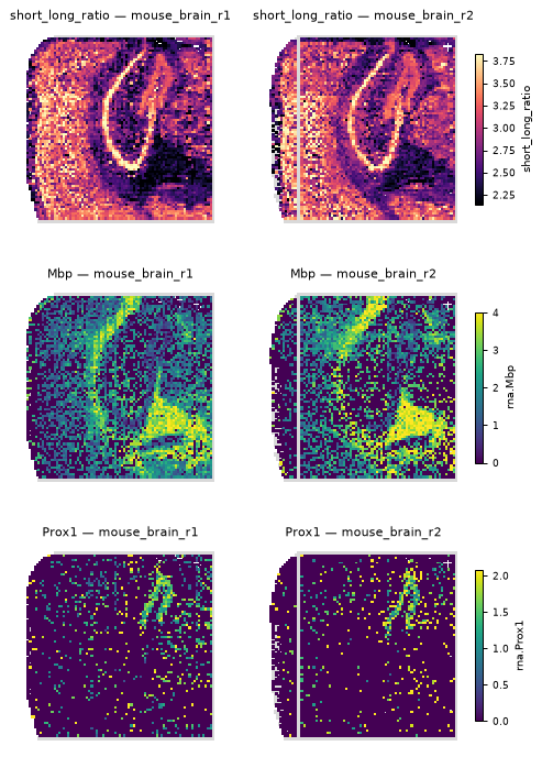
Regions from marker sets of the spot RNA, smoothed over the spot’s neighbours (cortex, CA, DG, white matter, choroid plexus, thalamus; a spot is left other when no set stands out), and the paper’s statement: the ratio is higher in cortex, CA and DG than in white matter and the choroid plexus.

markers = {"white_matter": ["Mbp", "Plp1", "Mog", "Cldn11", "Mal"], "choroid_plexus": ["Ttr", "Kl"],
           "DG": ["Prox1"], "CA": ["Neurod6"], "cortex": ["Satb2", "Cux2", "Rorb", "Fezf2"],
           "thalamus": ["Slc17a6"]}
from scipy.spatial import cKDTree
region = pd.Series("other", index=c.index)
for sec, g in c.groupby("section", observed=True):
    score = pd.DataFrame({r: g[[f"rna.{m}" for m in ms if f"rna.{m}" in g]].mean(axis=1) for r, ms in markers.items()})
    nb = cKDTree(g[["centroid_x", "centroid_y"]].to_numpy()).query_ball_point(g[["centroid_x", "centroid_y"]].to_numpy(), r=2.01)
    sm = np.array([score.to_numpy()[n].mean(0) for n in nb])
    z = (sm - sm.mean(0)) / sm.std(0)
    region[g.index] = np.where(z.max(1) > 0.5, np.array(list(markers))[z.argmax(1)], "other")
c["region"] = region
q = c[c.qc]
print(q.groupby(["section", "region"], observed=True)["short_long_ratio"].median().unstack(0).round(2))
for sec, g in q.groupby("section", observed=True):
    hi = g[g.region.isin(["cortex", "CA", "DG"])].short_long_ratio
    lo = g[g.region.isin(["white_matter", "choroid_plexus"])].short_long_ratio
    u = stats.mannwhitneyu(hi, lo, alternative="greater")
    print(f"{sec}: cortex/CA/DG median {hi.median():.2f} vs white matter/choroid plexus {lo.median():.2f}, "
          f"AUC {u.statistic / (len(hi) * len(lo)):.2f}")

section         mouse_brain_r1  mouse_brain_r2
region                                        
CA                        3.13            3.13
DG                        2.90            2.95
choroid_plexus            2.49            2.54
cortex                    3.24            3.26
other                     2.91            2.92
thalamus                  2.89            2.94
white_matter              2.47            2.56
mouse_brain_r1: cortex/CA/DG median 3.13 vs white matter/choroid plexus 2.48, AUC 0.86
mouse_brain_r2: cortex/CA/DG median 3.14 vs white matter/choroid plexus 2.56, AUC 0.86

3. Barcode stripes

Every array row and every column is barcoded through its own channel: a channel’s efficiency adds an offset to all its spots. destripe fits the row and column offsets together with a smooth surface (cubic B-splines, knots every 6 spots) and removes only their rough part — the jumps between neighbouring rows / columns; the smooth pattern (anatomy, and a slow drift that cannot be told apart from it) stays. The depth of the spots shows the stripes best.

g = q[q.section == "mouse_brain_r1"]
rows, cols = g.centroid_y.to_numpy(int), g.centroid_x.to_numpy(int)
ds_ = destripe(g[["log_contacts", "short_long_ratio", "cis_fraction", "frac_2M_12M"]], rows, cols)
fig, axes = plt.subplots(1, 2, figsize=(7, 3.4))
plot_spatial(cd, g["log_contacts"], ax=axes[0], title="log10 contacts")
plot_spatial(cd, ds_["log_contacts"], ax=axes[1], title="destriped")
plt.show()
xy = g[["centroid_x", "centroid_y"]].to_numpy(float)
print("smooth share of the variance, raw -> destriped:",
      dict(zip(ds_.columns, zip(smooth_share(g[ds_.columns], xy).round(2), smooth_share(ds_, xy).round(2)))))

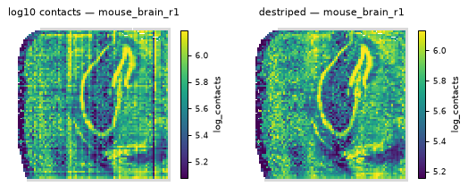
smooth share of the variance, raw -> destriped: {'log_contacts': (np.float64(0.45), np.float64(0.56)), 'short_long_ratio': (np.float64(0.57), np.float64(0.59)), 'cis_fraction': (np.float64(0.67), np.float64(0.69)), 'frac_2M_12M': (np.float64(0.62), np.float64(0.64))}

4. Spatial tests, raw and adjusted

Per section: Moran’s I over the 8 adjacent spots, and SPARK-X (eleven coordinate kernels, Cauchy-combined, Benjamini–Yekutieli over features) on the destriped values — raw, with the spot’s depth, and with depth + the 30 RNA principal components of the store (cellm["rna_pca"]). The share of the smooth spatial variance that is left after each adjustment is the effect size; with ~6,000 spots every p-value is tiny. The undigested / self-ligated share (contacts under 2.5 kb) is a library QC value: a contrast that the RNA should not explain.

o = cd.cellm["contacts.orientation"].astype(float)
c["frac_lt2k5"] = o[:, :, 0].sum(1) / o.sum((1, 2))       # histogram column 0: d < 2.5 kb
q = c[c.qc]
pcs = pd.DataFrame(np.asarray(cd.cellm["rna_pca"]), index=c.index)
feats = ["short_long_ratio", "frac_2M_12M", "ps_slope_1M_10M", "cis_fraction", "frac_lt2k5"]

def resid(v, X):
    Xi = np.c_[np.ones(len(v)), X]
    b, *_ = np.linalg.lstsq(Xi, v, rcond=None)
    return v - Xi @ b

rows_ = []
for sec, g in q.groupby("section", observed=True):
    xy = g[["centroid_x", "centroid_y"]].to_numpy(float)
    D = destripe(g[feats], g.centroid_y.to_numpy(int), g.centroid_x.to_numpy(int))
    dep = g[["log_contacts"]].to_numpy()
    P = pcs.loc[g.index].to_numpy()
    graph = spatial_neighbors(cd, method="radius", radius=1.5, cells=g.index)
    base = smooth_share(D, xy) * D.var().to_numpy()
    for name, X in (("raw", None), ("depth", dep), ("depth + RNA", np.c_[dep, P])):
        R = D if X is None else pd.DataFrame({k: resid(D[k].to_numpy(), X) for k in feats}, index=g.index)
        I = spatial_autocorr(values=R, graph=graph)["I"]
        left = smooth_share(R, xy) * R.var().to_numpy() / base
        sx = sparkx(D, xy, covariates=X)
        for k in feats:
            rows_.append({"section": sec, "adjusted for": name, "feature": k, "Moran I": I[k],
                          "smooth variance left": left[feats.index(k)], "SPARK-X padj": sx.loc[k, "padj"]})
res = pd.DataFrame(rows_)
res.pivot_table(index=["feature", "adjusted for"], columns="section",
                values=["Moran I", "smooth variance left"]).round(3)

		Moran I		smooth variance left
	section	mouse_brain_r1	mouse_brain_r2	mouse_brain_r1	mouse_brain_r2
feature	adjusted for
cis_fraction	depth	0.744	0.623	1.010	1.007
	depth + RNA	0.361	0.275	0.192	0.199
	raw	0.737	0.619	1.000	1.000
frac_2M_12M	depth	0.676	0.598	0.964	0.983
	depth + RNA	0.266	0.204	0.136	0.149
	raw	0.683	0.600	1.000	1.000
frac_lt2k5	depth	0.588	0.650	0.802	0.919
	depth + RNA	0.470	0.515	0.464	0.579
	raw	0.668	0.672	1.000	1.000
ps_slope_1M_10M	depth	0.643	0.572	0.911	0.950
	depth + RNA	0.190	0.169	0.090	0.124
	raw	0.669	0.586	1.000	1.000
short_long_ratio	depth	0.605	0.546	0.904	0.948
	depth + RNA	0.194	0.169	0.104	0.131
	raw	0.630	0.558	1.000	1.000

The contact features vary strongly in space (Moran’s I 0.5–0.7), and the spot’s transcriptome accounts for most of it: about a tenth of their smooth spatial variance is left after the RNA, while the library QC value keeps about half. Is the tenth that is left 3-D genome variation beyond the cells? An adjustment by noisy covariates is never complete, so it needs a yardstick: genes held out of the RNA components, adjusted the same way. uchrom-reproducibility extended_data_fig2 (stage calibrate) does this on the full transcriptome: spatially patterned held-out genes keep about 30 % of their smooth variance, more than the contact features keep. On these data the global 3-D genome features follow the cells at least as closely as the cells’ other genes do.

Next: the same tests for known structures scored in every spot — boundary insulation and loop strength from contacts counted in their windows (uchrom.io.WindowCounts, uchrom.fea.window_scores) and compartment values (uc.tl.single_cell_compartments) — in spatial variation across a tissue.